A famous 17th century defender of the newly emergent Scientific Revolution, Francis Bacon in his 1620 book Novum Organum also warned about the four main ways that we can obstruct truth. One of these obstructions is called the “Idols of the Marketplace,” which is how our imprecise and deceptive use of language may blind us. Even a relatively minor misuse of words may create an idol, as it were, that we worship by mindlessly repeating a phrase that obstructs truth in some way. I was reminded of the “Idol of the Marketplace” in the specific phrase often repeated in Tensor Calculus: that parallel transporting vectors is the mechanism behind the Riemann curvature tensor. However, most derivations of the Riemann Tensor say that we are parallel transporting vectors without ever explicitly including the parallel transport equation, as if the vectors parallel transport by magic. In order to understand how the Riemann Tensor actually can employ parallel transport, parallel transport itself must be the starting point of the derivation. Then we will prove that the traditional derivations which neglect the parallel transport equation implicitly include parallel transport within the definition of the covariant derivative.
Therefore, this post has three main aims:
- To introduce some of the basics behind tensor calculus in an intuitive, visual way in order to :
2.Show how and why parallel transport can be made explicit in a derivation of the Riemann Curvature tensor
3. To show that the traditional derivations of the Riemann tensor employ the covariant derivative, which embeds the definition of parallel transport within it.
Because of these aims, a familiarity with tensor calculus is assumed, though it may not be strictly necessary as I will try to explain some of the mathematics of tensors.
Part I: TENSOR CALCULUS INTRODUCTION– Christoffel Symbols, Parallel Transport and the Covariant Derivative (note that a much more extensive introduction is available in the Appendix for those who have less familiarity with tensor calculus)
Christoffel symbols
Christoffel symbols measure how the basis vectors change over a given coordinate:

the symbol


So

As we move in the


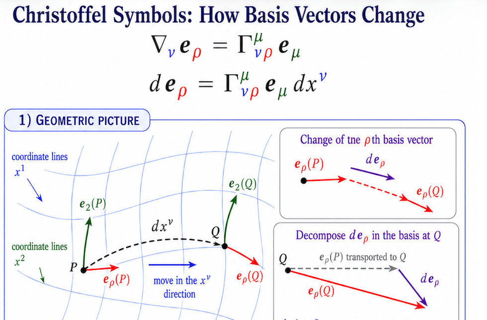
Note that dep signifies the change in the basis vector, and then we would simply divide by dxv to show the change of dep over our chosen differential dxv (which is usually infinitesimal).
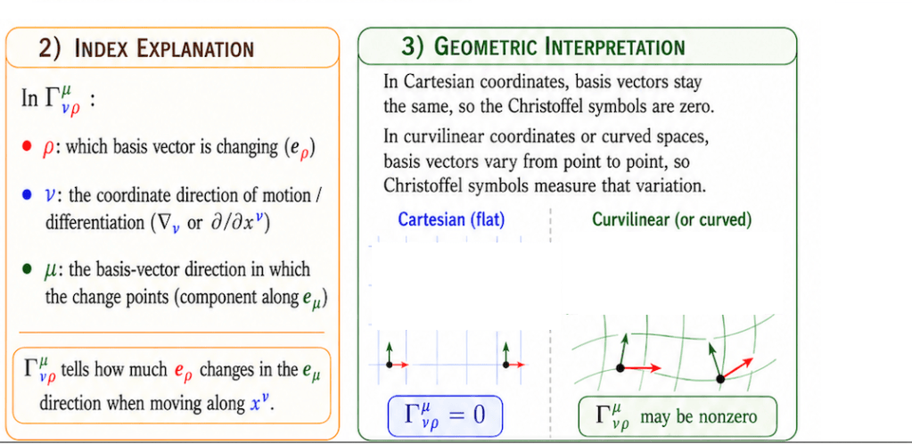
In the above we see that we moved 


In plain language, the Christoffel symbols measure how the coordinate grid itself twists, stretches, or turns from point to point. They are not measuring a new physical force by themselves. They are measuring how our local basis vectors change as we move. Note that the Christoffel symbol may be non zero when the coordinate system is curvilinear, even in a flat space. However, if the underlying space is flat and we are using Cartesian coordinates, the Christoffel symbol would be 0 because there is no directional or component change in the basis vectors.
In summary, the whole reason why the Christoffel symbols appear in the covariant derivative is that we have to account for two kinds of change: the vector’s components may change, and the basis vectors themselves may change. The Christoffel symbol supplies the correction for the changing basis.
Covariant Derivative
Before delving into how tensor calculus can help us understand curvature of space, we must first define how we take a derivative of a vector. Because the vector has two multiplicative parts, the component and the basis vector, we must apply the product rule when we differentiate, because not only the component might be changing but also the basis vectors themselves may be changing! The derivative of a vector (expressed as the sum of the linear combinations of all its contravariant components and covariant bases) is known as the covariant derivative.

Now dot both sides with the contravariant basis vector:
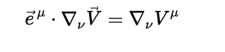
so that we extract the contravariant u component on the left side and cancel the covrariant base with the contravariant base on the right side:


When the covariant derivative of a vector is 0, we get the condition for parallel transport:
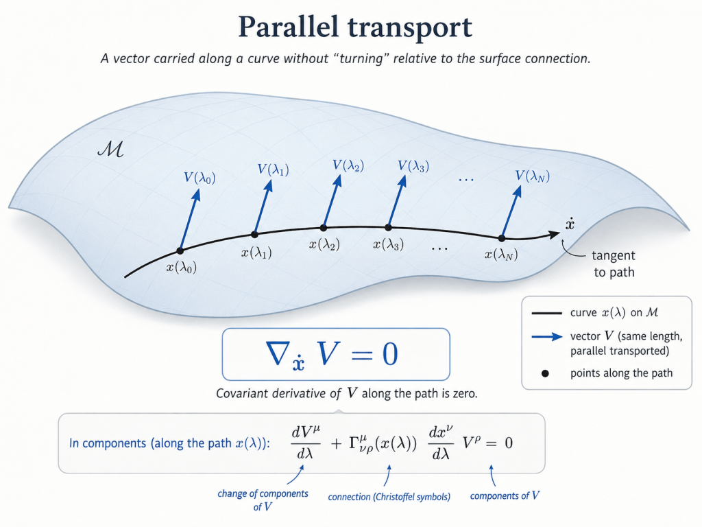
This means that as we nudge a vector an infinitesimal distance in the v coordinate direction, we do not change the vector at all; even if the underlying basis changes, the components will change in exactly the opposite way to result in 0 net change of the vector.
We see that there is an extra term in the formula compared to the covariant derivative , namely 
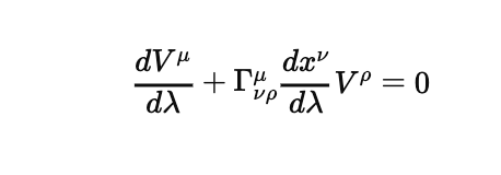
When the vector and the coordinate system itself are written in terms of the parameter 
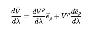
and then by use of the chain rule we have
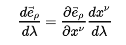
where
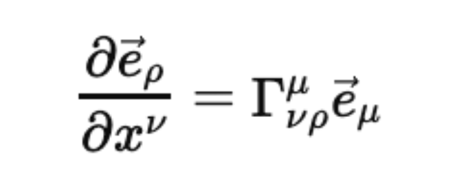
so
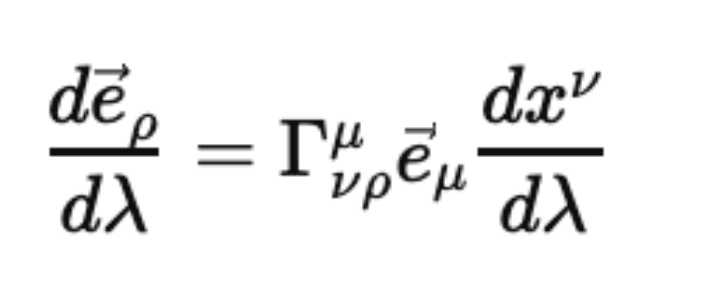
leading us back to
Part II: The Riemann Curvature Tensor
Below is the formula for the Riemann Curvature Tensor:
This scary looking formula is first best understood with the basic intuitions shown in the pictures below
In flat space, ordinary partial derivatives commute when applied to vectors tangent to a surface (to understand why, please visit https://mathintuitions.com/2025/05/27/divergence-curl-and-the-taylor-series-approximation/ in order to get the intuition behind Clairaut’s theorem):

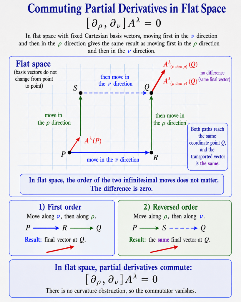
This means that if we first move in the ν direction and then the ρ direction, or first move in the ρ direction and then the ν direction, the result is the same. The coordinate system can be any shape, but the fact that the underlying space is flat will always be reflected by the partial derivatives commuting.
But in curved space, the partial derivatives do not commute when applied to tangent vectors:
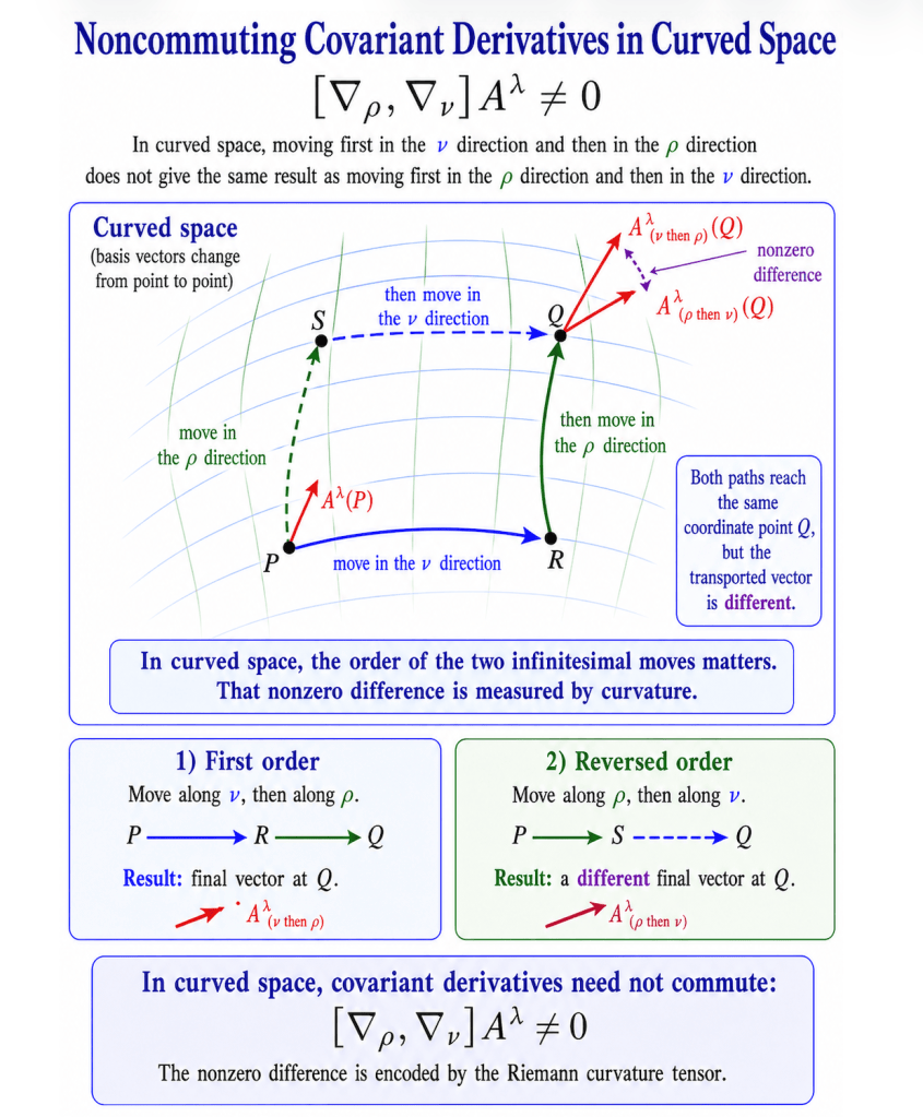
So the Riemann tensor measures the failure of covariant derivatives to commute:
This is why the Riemann tensor is the mathematical object that captures intrinsic curvature. It tells us whether moving in one direction and then another gives the same result as moving in the opposite order. If the result depends on the order, the space is curved.
You may notice that the common derivation of the Riemann Curvature Tensor lacks the definition of parallel transport, despite the fact that it is often claimed in the same derivation that parallel transport is used.
Our goal is to clearly show that the Riemann Tensor is derived through parallel transporting a tangent vector around a loop, through starting with the very definition of parallel transport itself and clearly incorporating it from the start in our derivation.
Recall that we derived our parallel transport equation earlier as:
Next we want to understand how the vector components alone change under parallel transport (the components alone will record the meaningful change, since the basis vectors begin and end at the same point) so we start by subtracting the Christoffel symbol term:
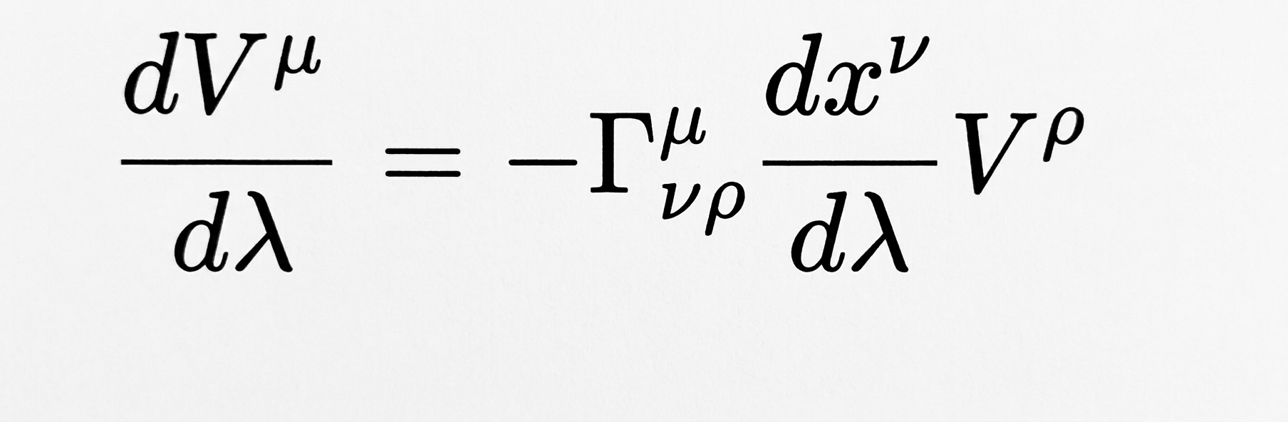
To isolate the change in the vector components under parallel transport , we multiply by dgamma:
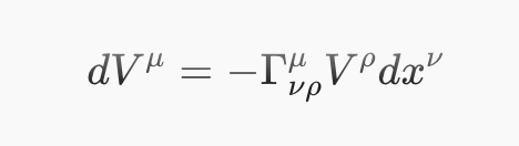
The above equation looks scary, but the intuition is simple: it is saying that the change in the vector components is equal to the rate of change that is opposite to the basis vectors (shown by the Christoffel symbol), , multiplied by the number of steps we apply that change (shown by dxv), multiplied by the initial component amount of the vector (the Vp). To make this more concrete, if for a given component in a given direction the basis vector changes by 2, then that modifies every unit of a vector by -2, times the number of steps across that direction (in this case, the infinitesimal amount dx).
We will explicitly show how the tangent vector Vp (tangent to surface but can be pointing in any direction on surface) is first transported along v then sigma and then vice versa.
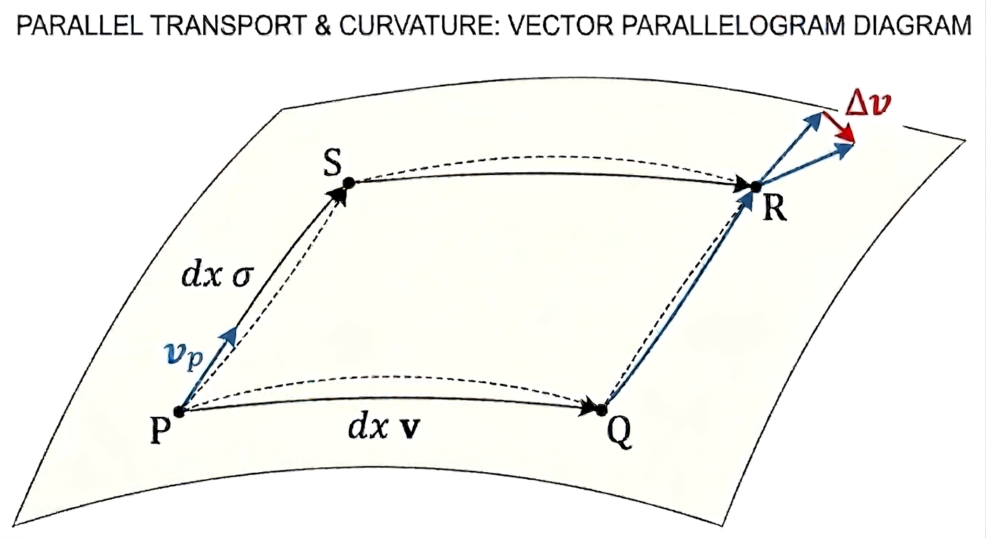
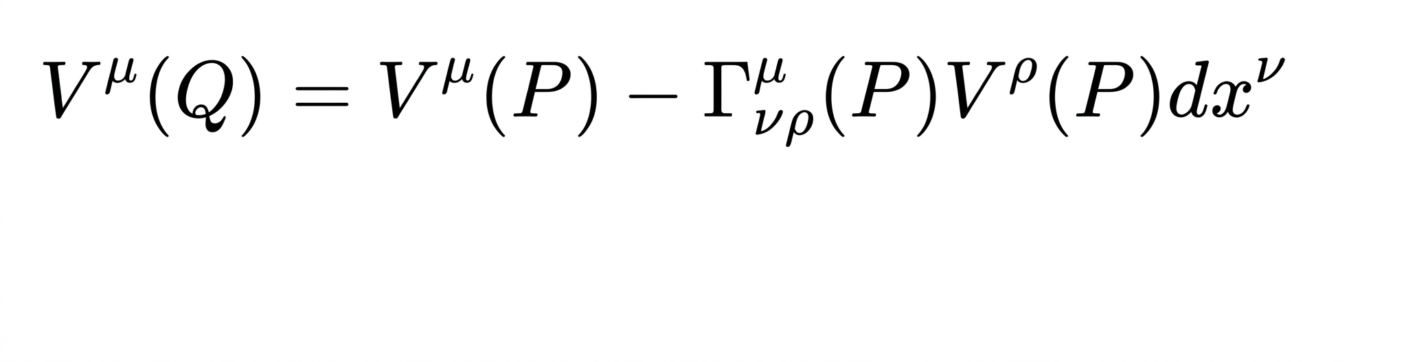
We know that to get the vector at point Q, we can move the vector at P by an infinitesimal amount across to point Q where the original vector at P changes by dVu, so: Vu(Q)= Vu(P) + dVu. Now we substitute the above equation for dVu, which ensures that the vector at P is parallel transported to Q across dxv.
Now we want to move the vector we parallel transport to point Q up across the sigma coordinate to R, so we start with:
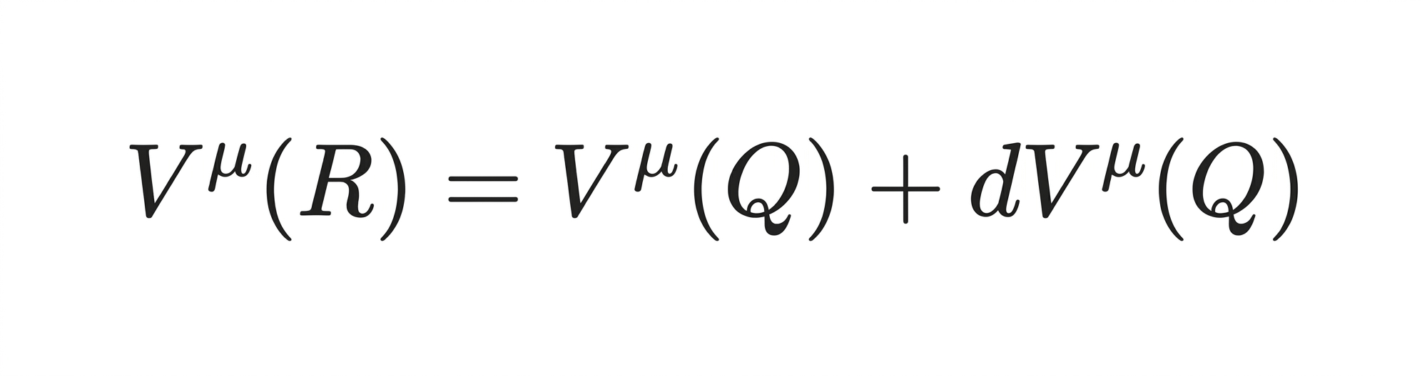
and once again impose that our dV meets the parallel transported condition of
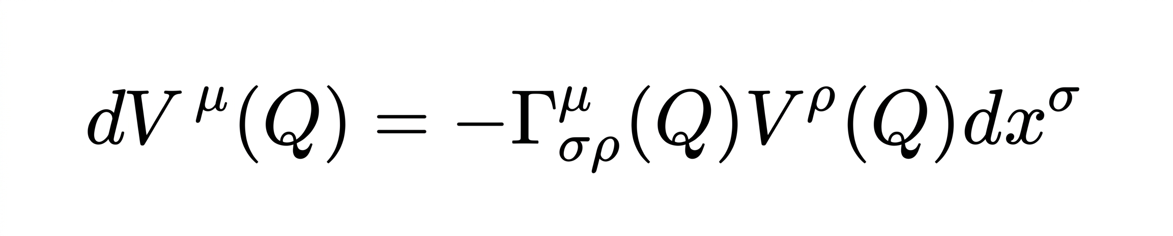
and substituting we get:

We don’t know the Christoffel symbol or vector values at point Q, so we must use the known values for both at point P and estimate what they would be at point Q through a Taylor series expansion centered at point P. Here is the Taylor series estimate for the Christoffel symbol at point Q using the known value at point P and transporting it from P to Q (where dxv= X-P)

We can ignore the second order term above since it is infinitesimally smaller than our first infinitesimal term, and when multiplied by the dx at the end of the factor would give us a 3rd order term (we are ultimately only interested in terms up to second order), and we can now plug this estimation for the Christoffel symbol at point Q back into our equation for V(R) , where the estimation appears in the parentheses:

We now want to replace our V(Q)’s with our previously calculated expression for V(Q), which showed that it was parallel transported from point P to Q:
![\displaystyle V^\mu(R) \approx \left[ V^\mu(P) - \Gamma^\mu_{\nu\lambda}(P) V^\lambda(P) dx^\nu \right] - \left( \Gamma^\mu_{\sigma\rho}(P) + \partial_\nu \Gamma^\mu_{\sigma\rho}(P) dx^\nu \right) \left[ V^\rho(P) - \Gamma^\rho_{\nu\lambda}(P) V^\lambda(P) dx^\nu \right] dx^\sigma](https://s0.wp.com/latex.php?latex=%5Cdisplaystyle+V%5E%5Cmu%28R%29+%5Capprox+%5Cleft%5B+V%5E%5Cmu%28P%29+-+%5CGamma%5E%5Cmu_%7B%5Cnu%5Clambda%7D%28P%29+V%5E%5Clambda%28P%29+dx%5E%5Cnu+%5Cright%5D+-+%5Cleft%28+%5CGamma%5E%5Cmu_%7B%5Csigma%5Crho%7D%28P%29+%2B+%5Cpartial_%5Cnu+%5CGamma%5E%5Cmu_%7B%5Csigma%5Crho%7D%28P%29+dx%5E%5Cnu+%5Cright%29+%5Cleft%5B+V%5E%5Crho%28P%29+-+%5CGamma%5E%5Crho_%7B%5Cnu%5Clambda%7D%28P%29+V%5E%5Clambda%28P%29+dx%5E%5Cnu+%5Cright%5D+dx%5E%5Csigma&bg=eeeeee&fg=666666&s=0&c=20201002)
We can distribute our dx sigma at the end of the equation to the final two terms and then expand the product:
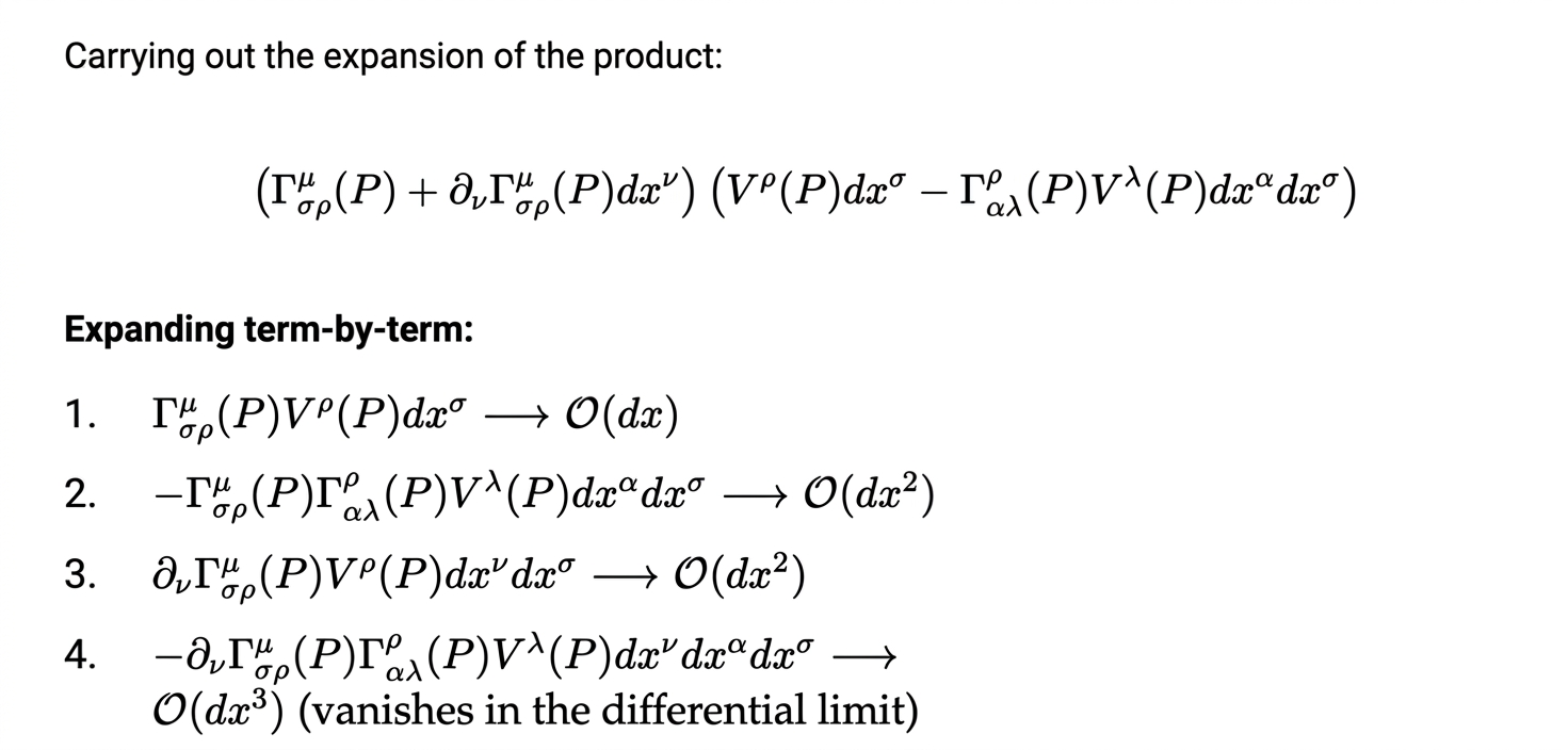
Dropping terms higher than 3rd order gives us our final expression:
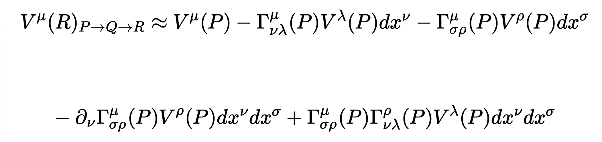
Now we simply switch the sigma and v positions in the above equation to get the final vector first transported up along dx sigma and then across dxv (parallel transporting from P to S to R), since it is derived by the same process just with a different order of the coordinate indices:
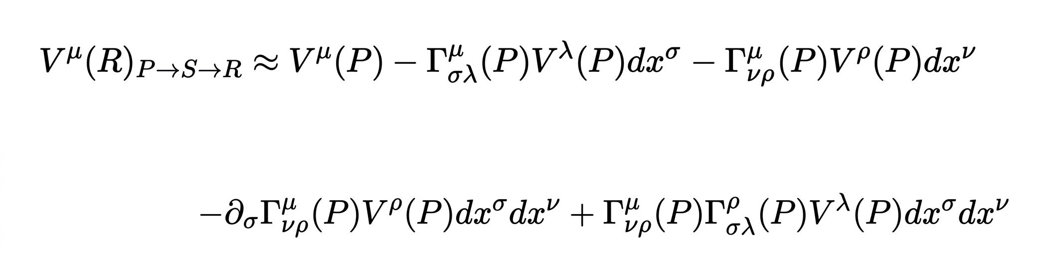
Next, we want to subtract the second vector (the one transported from P to S to R) from the first vector (the one transported from P to Q to R) in order to see the change in the vector due to the different paths taken (flat surfaces will show no difference). This will give us the Riemann Curvature Tensor: after performing the following three steps:
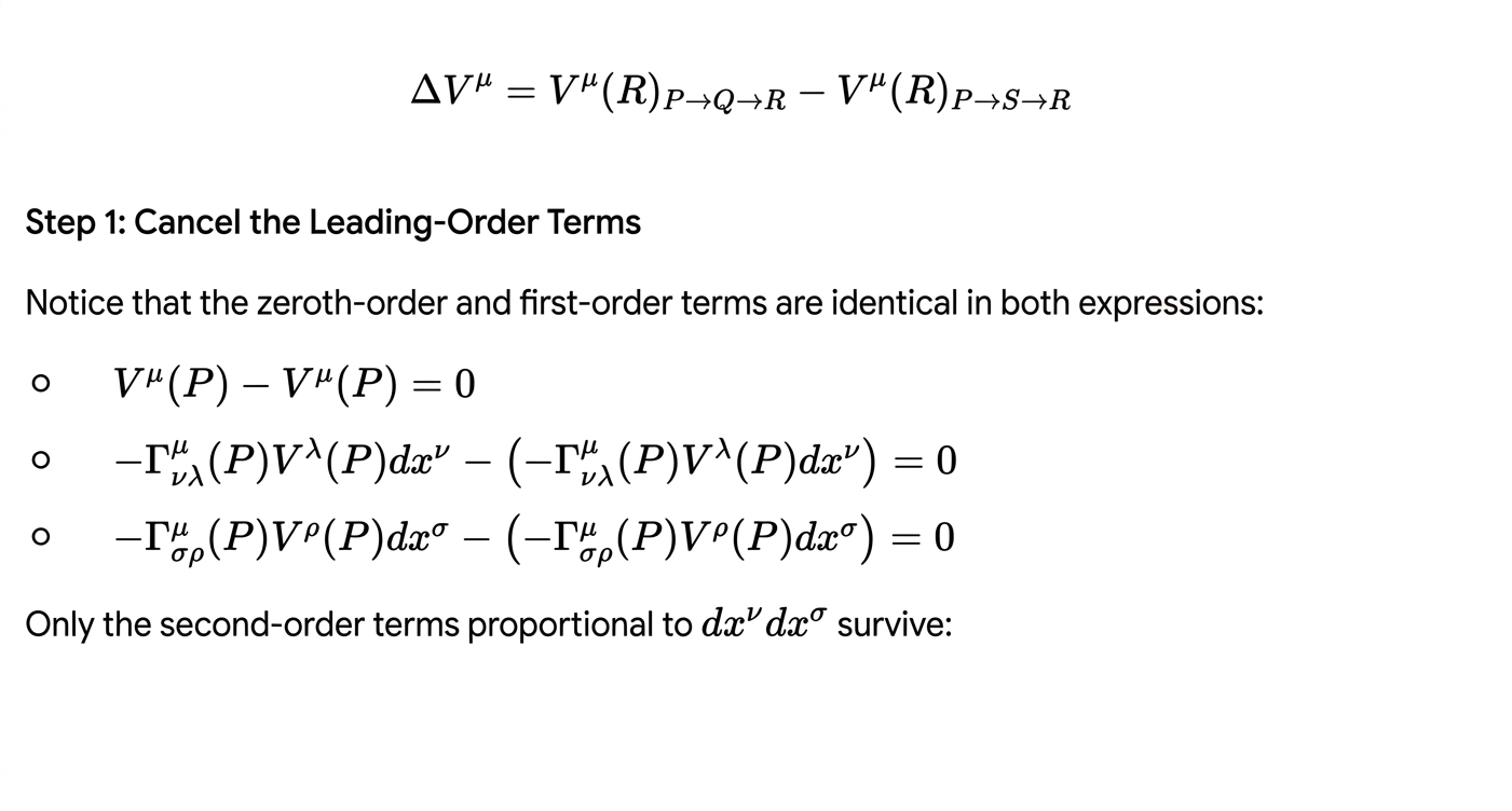

For the second steps, we will relabel the dummy indices in order to factor out the vector component Vp .
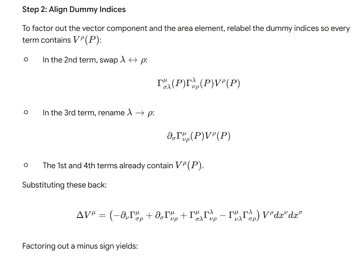
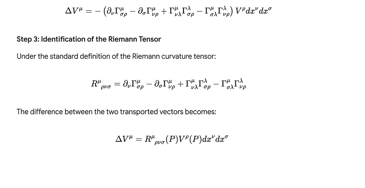
Note that if we had subtracted the first vector from the second, we wouldn’t have needed to factor out the negative sign, and would have still been left with the same definition as above. This proof above shows that we can derive the Riemann Tensor by starting with the parallel transport definition.
However, the typical derivation of the Riemann Tensor does not make parallel transport explicit at all. This derivation is often used by those who claim that the Riemann Tensor is achieved by parallel transporting a vector, though the parallel transport equation is nowhere evident. We assume that our coordinates are u and v (instead of sigma and v shown above) and we first move in the v direction followed by the u direction and then subtract the movement in the u direction followed by the v direction, with a chosen vector component Vp. Note that below we are also using different index notations than the above in certain spots, but the math is still the same:
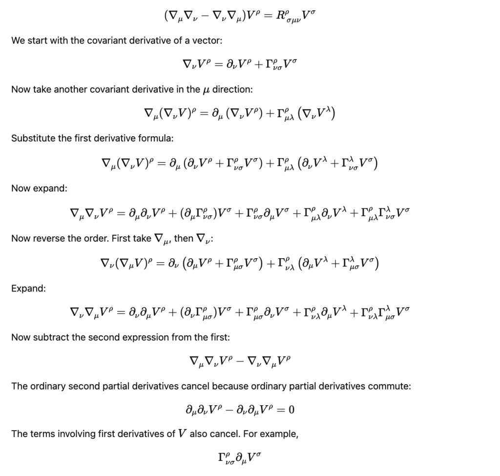
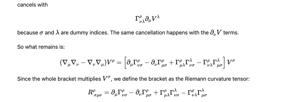
What the above derivation is telling us is that by applying covariant derivatives to a pre-existing vector field and moving around a loop in 2 different routes, we get the same result as if we parallel transported a single vector around the loop in 2 different routes.
So, how does the Riemann Tensor derived in the traditional way with covariant derivatives still achieve the same result as the Riemann Tensor derived with parallel transport?
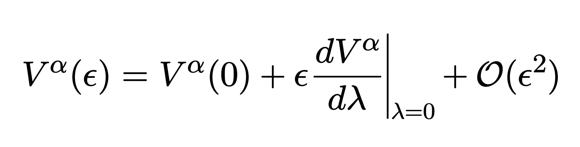
To understand why the application of the covariant derivative achieves the same result as parallel transporting in the Riemann Tensor, we can understand how the covariant derivative actually embeds parallel transport in its definition. First we will estimate a neighboring vector displaced by an infinitesimal distance epsilon in a vector field using the Taylor series around the point where lambda equals zero:
Now, let’s understand the parallel transported version of the above; as we already know, our definition of parallel transport means that (xo is where lambda is 0):

Next we plug the above into our first expansion to get the parallel transported version:

which implies that the parallel transported vector, up to first order, is equivalent to:

We now subtract the parallel transported vector from the original vector expansion , utilizing the chain rule so that we get the change in terms of lambda:

The above shows us the difference between the (estimated) vector in the vector field after traversing distance epsilon and the (estimated) parallel transported vector after traversing distance epsilon.
If we cancel terms, factor , and divide by epsilon we get:
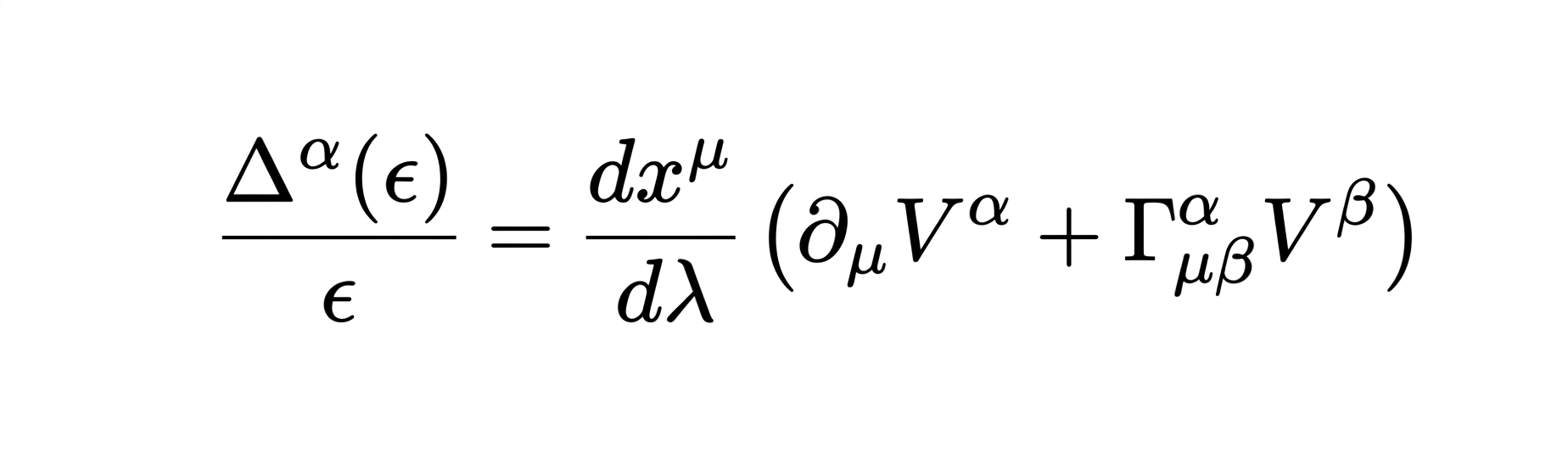
Note that the term in parentheses is the very definition of the covariant derivative!
Then, by taking the limit, we actually get our directional covariant derivative:
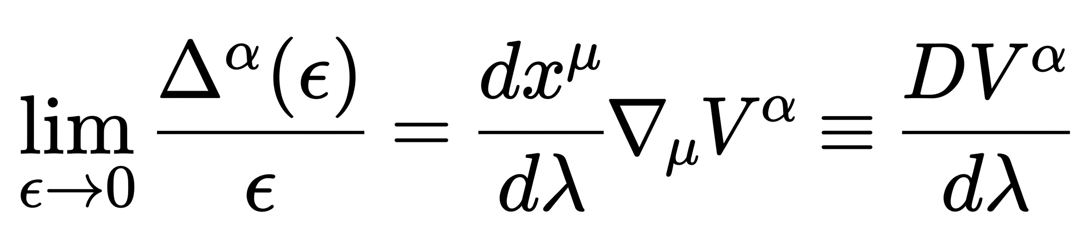
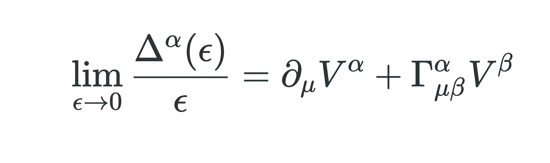
This is the definition of the directional covariant derivative, measuring the rate of change of a chosen vector component as it travels along the tangent vector parameterized by lambda. If we were to have moved along a single unparameterized coordinate line, we would get the standard definition of the covariant derivative (where lambda would be equivalent to dxu ):
All this leads to a profound discovery: that the covariant derivative is equal to the limit of the difference between the change in the vector field and its parallel transported version:

This equation implies that as we track the covariant derivative on 2 different routes around a loop, each with the same starting and ending point, the first term showing the change in vector components would be equivalent after taking both of the separate routes. The reason for this is that the first term represents just scalar vector components without a direction, so due to Clairaut’s theorem the mixed partial derivatives must be equal (please see my post at https://mathintuitions.com/2025/05/27/divergence-curl-and-the-taylor-series-approximation/ for the intuition behind this).
However, the second term of parallel transport would not stay equivalent at the end of each route on a curved surface. Thus, because the definition of the covariant derivative embeds parallel transport within tracking a preexisting vector field, we don’t have to parallel transport a single vector around a loop; rather we can simply take the covariant derivative around the loop and figure out if there is a difference at the end of each route, which would solely be attributable to the parallel transport term within the covariant derivative. This is why we would get that same value for the Riemann Tensor either by parallel transporting a single vector along 2 routes of a loop or by applying the covariant derivative along two routes of a preexisting vector field: the parallel transport within the covariant derivative is the only thing that detects curvature.
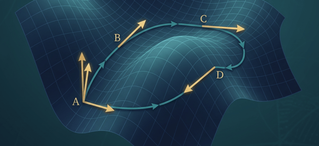
Most diagrams illustrating the Riemann curvature tensor, like the one below, actually show the parallel transport of a single vector around a loop, while using the traditional derivation of the Riemann Tensor that doesn’t quite match. Now we know that the traditional derivation in fact relies upon a preexisting vector field that is tracked with covariant derivatives, which embed the parallel transport that detects the curvature.
To sum up with a general intuition: no matter my coordinate system, as seen in the picture below, the 2 final parallel-transported vectors will be different from each other on a curved surface. The two final vectors differ because on the sphere, parallel transport around the loop produces a leftover rotation of the local tangent frame relative to the vector. That leftover, path-dependent frame rotation is what the Riemann tensor measures. Note that despite “seeming curved,” a cylinder is still flat because 2 parallel transported vectors are identical at the end of their separate paths. This is illustrated by the picture below:
.
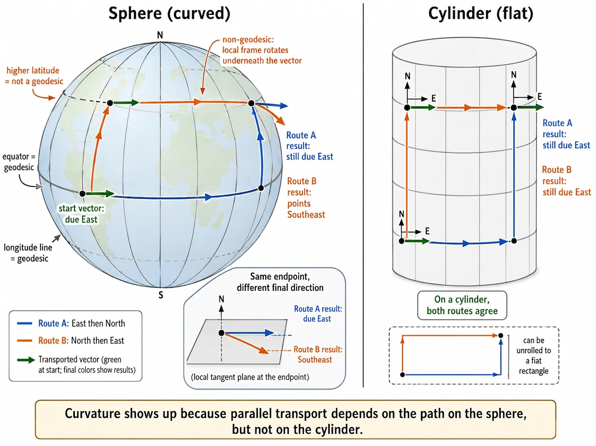
The cylinder curves through another extrinsic dimension, but intrinsically it is flat since you can unroll it into a flat sheet. If you live in the tangent space of the cylinder, there is never any turning or twisting of the tangent space, and therefore there is no curvature detected by the parallel transport of a vector.
Hopefully, we have removed the idol of the marketplace when it comes to the mindless repetition of the phrase that we parallel transport a vector when performing the operations behind the Riemann Tensor. Instead, as we have learned, the Riemann Tensor usually applies covariant derivatives to a pre-existing vector field, and we have discovered that within every covariant derivative there is a parallel transport term, which is the detector of curvature.
Below you will find a more extensive intro to Tensor Calculus for those less familiar with it, as well as some interesting derivations:
APPENDIX- 1– Tensor Calculus Intro
I will start by trying to define what a tensor is and why it is so important: a tensor is a mathematical object that transforms according to certain rules when changing coordinates. Tensors serve as the backbone of physics because frames moving at different velocities, in different gravitational fields, or differing in other factors may have different coordinates ascribed to their geometries, and tensor mathematics essentially allows us to calculate the same invariants, like space-time distance, no matter our coordinate system.
Scalar
The first term I wanted to define is scalar. A scalar can be a temperature field, since at every point you get the same number, no matter the coordinates used

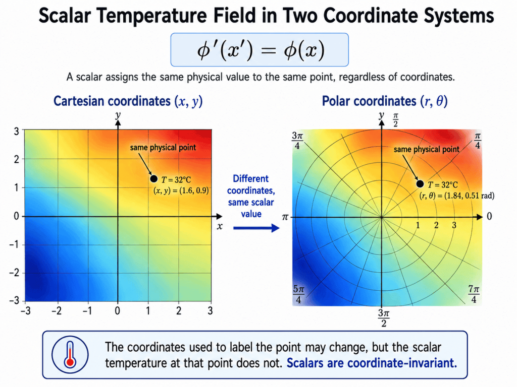
So given a coordinate transformation, we always get the same scalar value for a given point.
Contravariant Components
The second term I wanted to define is contravariant. We visited the example of the behavior of a contravariant vector in the previous post, https://mathintuitions.com/2026/05/20/the-metric-tensor-and-the-hidden-law-of-cosines/ and will review it again: imagine you have a basis vector of 1 meter pointing east, and you measure a distance of 1000 meters. Then, we rescale the basis vector so that it is now 1,000 times bigger; this new basis vector now represents 1 kilometer in a new coordinate system. What happens to our distance when we measure it in this new coordinate system? We now record 1 km of distance; this means that while we expanded the size of the basis vector by 1000, we shrunk the size of vector component by 1/1000, as in the following picture:
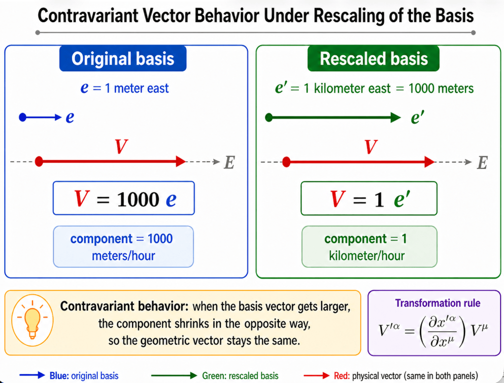
Vector components are contravariant because they behave in the opposite manner to the basis vectors upon scaling the basis vectors. The transform rule is 


At the same time, the basis vectors attached to the contravariant components actually transform covariantly, since, in our example above, it takes 1000 units of our original basis vector to equal to one unit of our new basis vector:, or in other words:
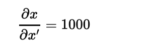
and generally we have
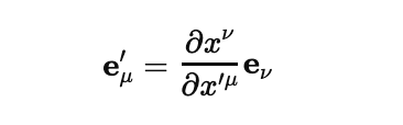
and now the u’ coordinate is in the denominator instead of the numerator of the transform.
Covariant Components
We have just touched on how covariant basis vectors are attached to contravariant components. However, components may also be covariant: the covariant component changes by the same factor as the covariant basis vector rather than by reciprocal factors. For example, if we measured a temperature field that got 1 degree hotter for every meter we moved due east, we would have a covariant component of 1 degree/meter. Now, if we then multiplied the physical length of the due east 1 meter covariant basis vector by 1000 to get a new basis vector of 1 km, we would also have multiplied our covariant component by a factor of 1000 to get 1000 degrees/1km since we would have traversed a greater difference in temperature by traversing a greater distance. Notice that when we increased the physical length of the covariant basis vector by a factor of 1,000, we also increase the covariant component by a factor of 1000. The rule for transforming a covariant vector in coordinate system v to the new coordinates in u’ is
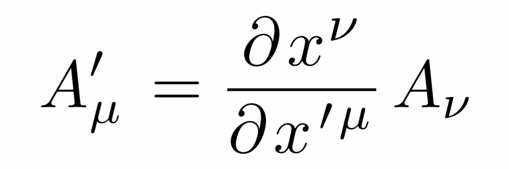
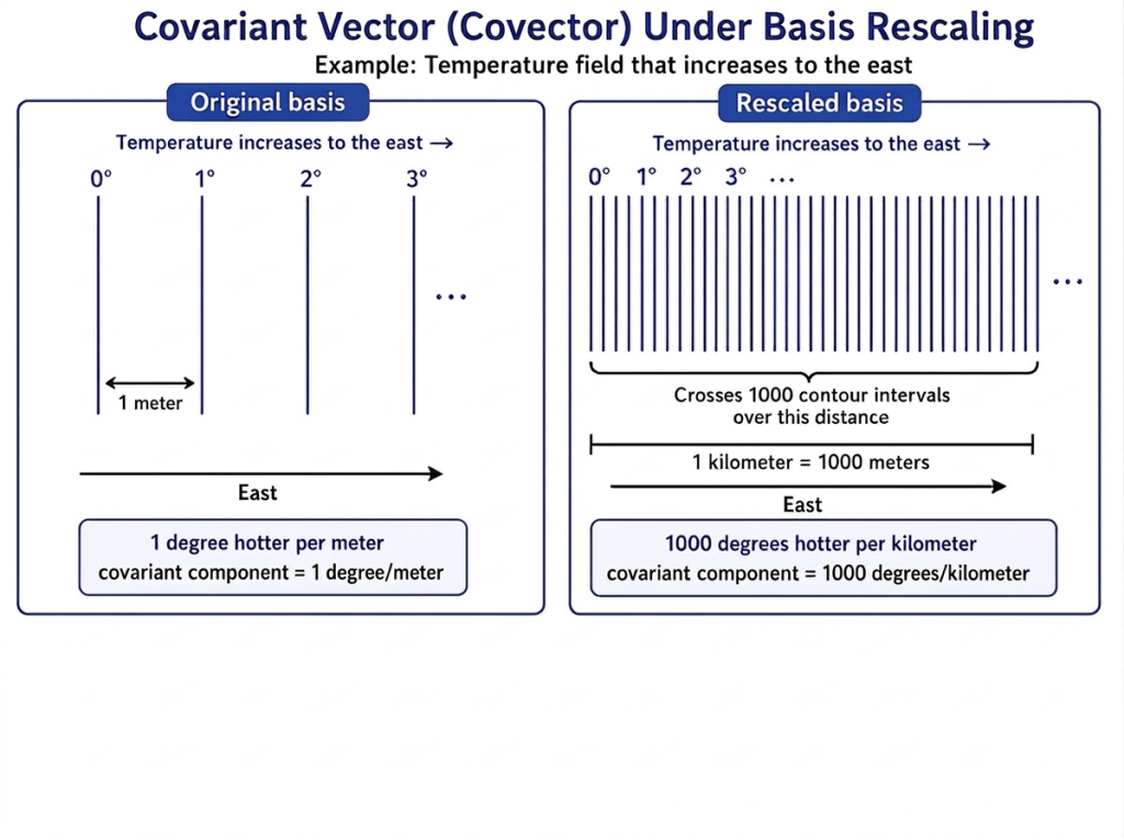
This means that the covariant component changes by the same factor as our original basis vector (original basis vector is the one we first created with the contravariant transform picture)!
As we change the basis vector from 1 meter to 1 km, we get the following differential transform 


our covariant transform is
where we know take the reciprocal of the contravariant transform, which is now:

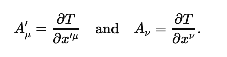
In the covariant general notation, the above transform an be written as

This matches
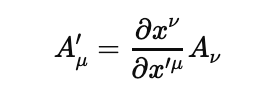
where
Covariant components are attached to contravariant bases, which are defined relative to the original covariant basis vectors. Each contravariant base is defined to be perpendicular to the covariant base of a different index, and it must also have a dot product of 1 with the covariant base of the same index:
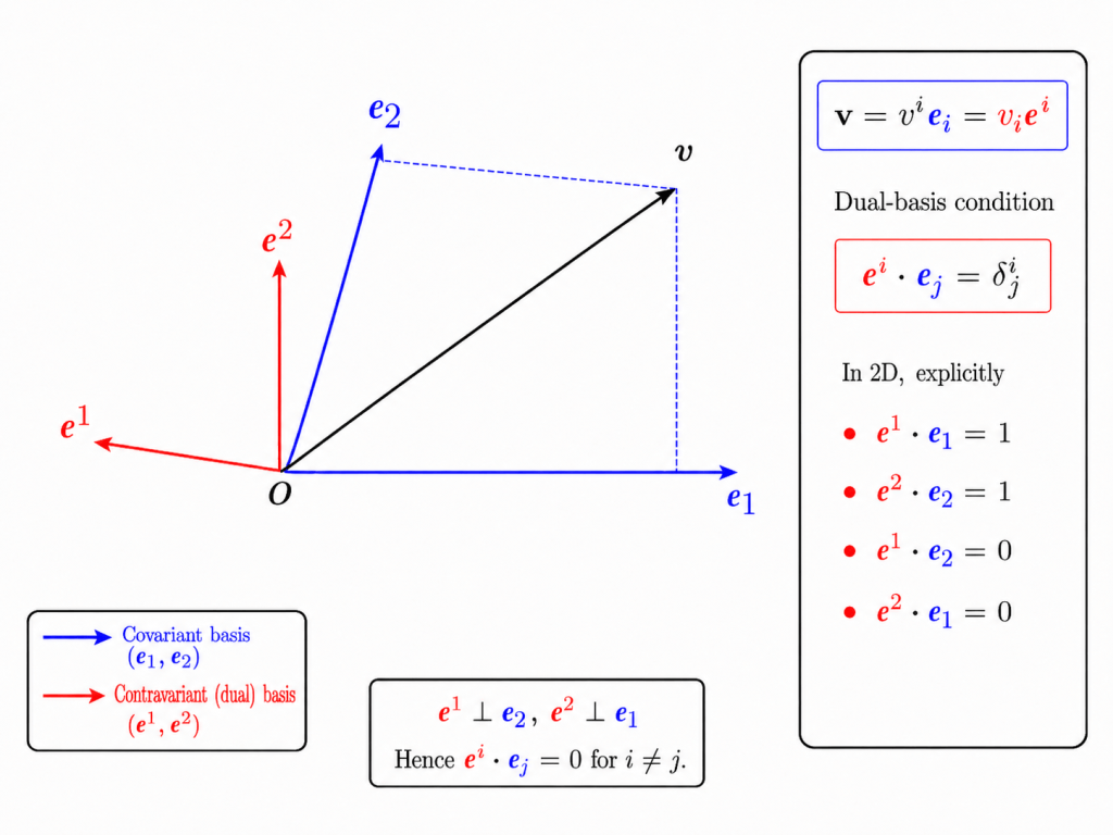
So vector v can be written equivalently with the contravariant components attached to covariant bases or covariant components attached to contravariant bases:

If we were dealing with 3 dimensions, we must still ensure that the dot products of bases with the same indices are 1 and that the bases with different indices are perpendicular to each other
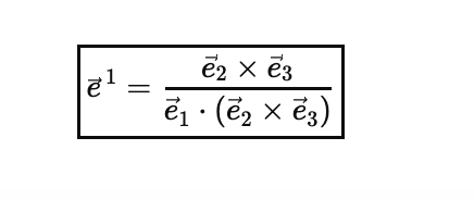
Note that the cross product term ensures the perpendicularity we require and then when we multiply each side by the dot product with e1 we ensure that the dot product of the two bases equals one (the cross product terms cancel).
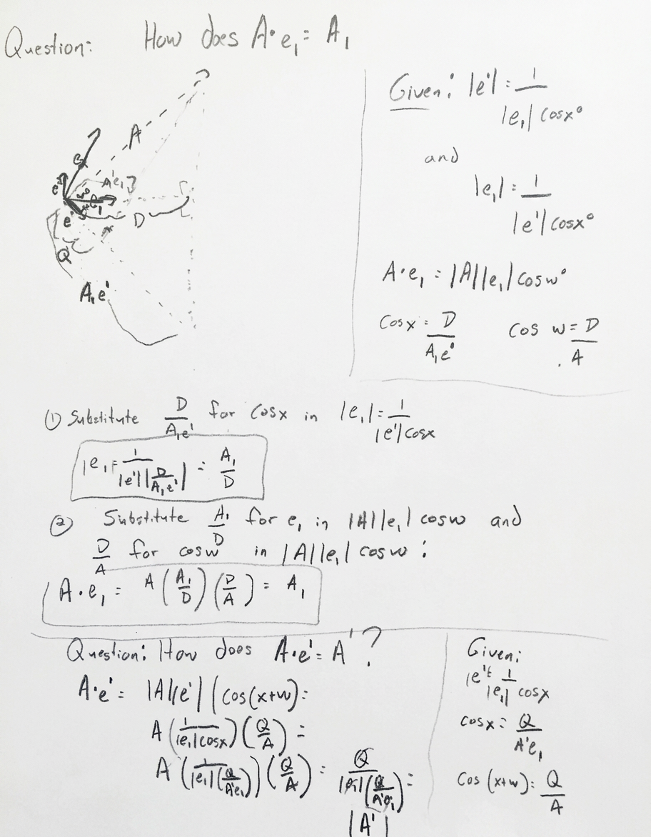
Now we will prove that
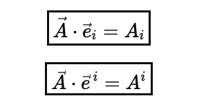
algebraically (for the geometric proof, please see the Appendix section towards the bottom of the post). Let’s start with proving the first equation:
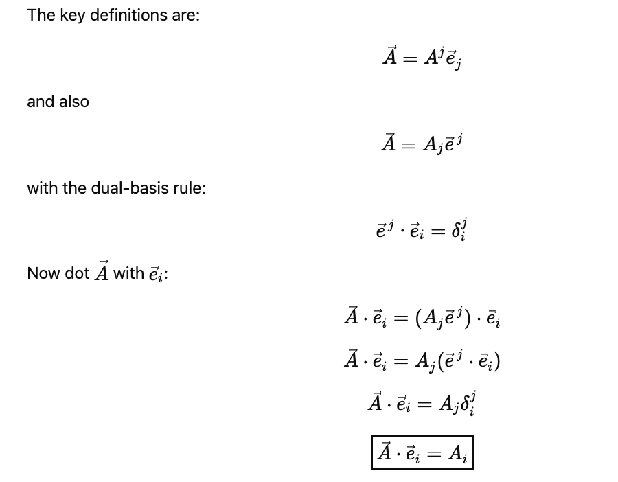
We can do the same to show the second rule by expressing A with its covariant base and contravariant component:
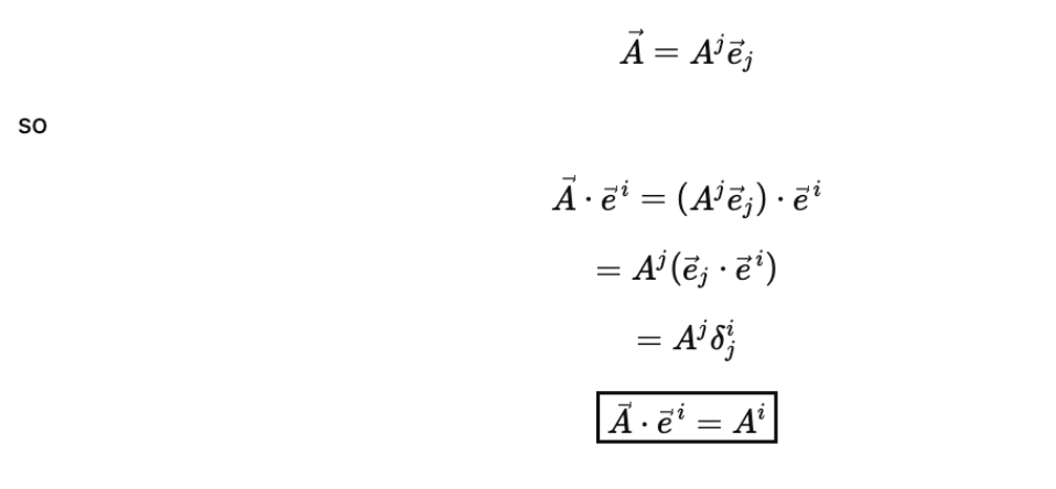
One of the main reasons we have the dual basis (contravariant basis vectors) in the first place is because of what the above shows: when taking the dot product of vector A with the dual basis, we can easily extract the contravariant component of the vector; likewise when taking the dot product of vector A with the covariant basis vector, we can easily extract the covariant component.
We also can very easily switch between different types of components components by either lowering or raising an index (in order to be covariant or contravariant, respectively) through the metric tensor, which is very useful for calculations (for more on the metric tensor, see the previous post https://mathintuitions.com/2026/05/20/the-metric-tensor-and-the-hidden-law-of-cosines/).
Now let’s see proof of the magic of how the metric tensor can help to raise or lower an index. We start with one of the definitions we just proved:
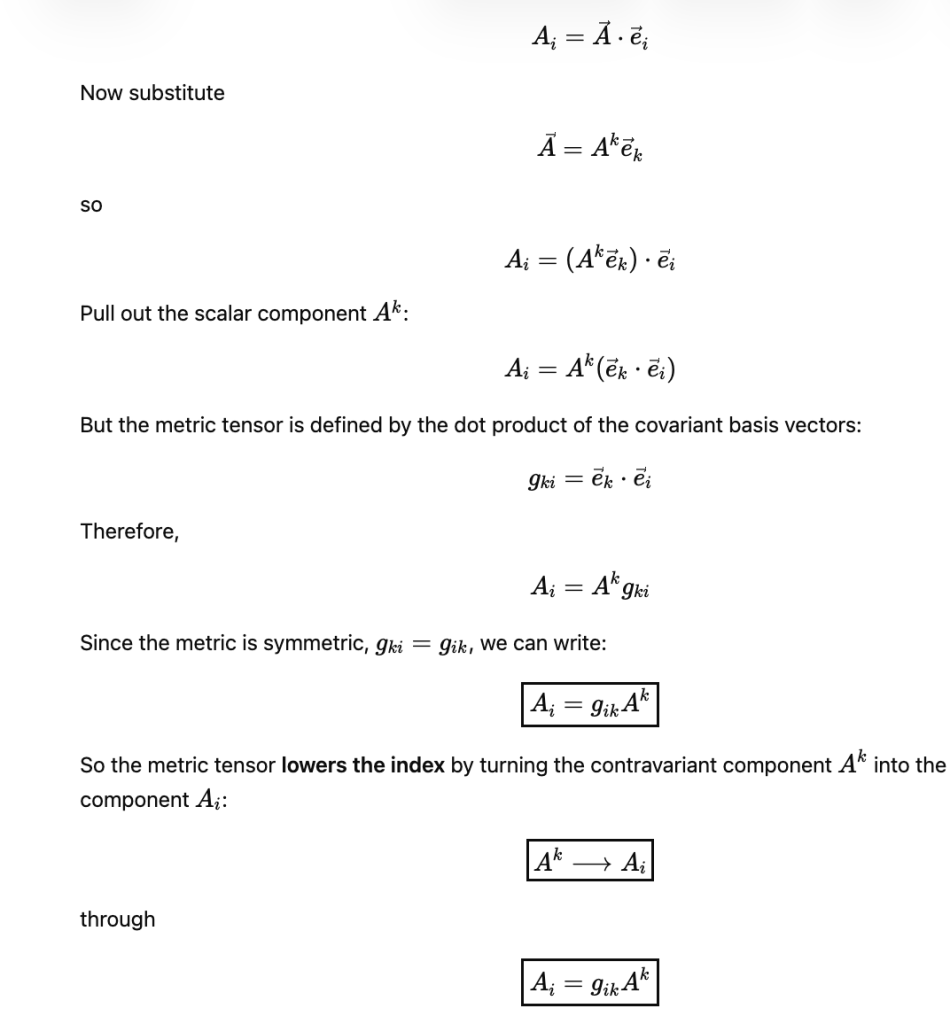
We have just proved how the metric tensor, summed over a contravariant component, can transform into the corresponding covariant component.
Now let’s show how we can raise an index to transform a covariant component into a contravariant component using a similar process:
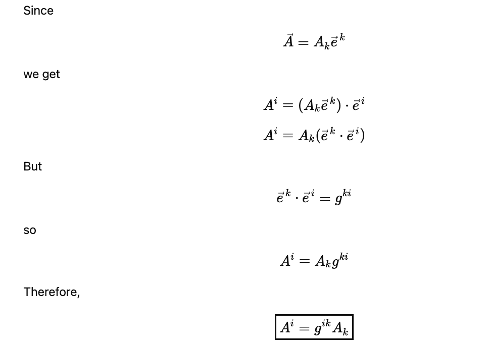
We have just proved how the metric tensor, summed over a covariant component, transforms into the corresponding contravariant component.
One other important idea about the nature of the different types of components is that a covariant component of a vector is needed along with a contravariant component in order to take the dot product. As we know from the previous post https://mathintuitions.com/2026/05/20/the-metric-tensor-and-the-hidden-law-of-cosines/, when we use the metric tensor in conjunction with the dot product of two vectors, we get a distance invariant whose basic foundation is the Law of Cosines and whose form is

Now our metric actually lowers the index of vector u and turns the equation into the multiplication of a covariant and contravariant component:

Now if the metric is the Cartesian metric whose basis vectors are of coordinate length 1 and orthogonal, we can simply multiply the two contravariant components together since the covariant and contravariant components are equal and the metric tensor is 1 for all indices that are the same and 0 for all indices that are different.
Mixed Tensors
We can also create mixed tensors, which have as many covariant and contravariant components as we choose. Below is an example of a 1,1 tensor (1 contravariant and 1 covariant component)

Covariant Derivative for a mixed tensor:


For a 1,1 tensor, the contravariant component’s basis vector has a + change, while the covariant component’s basis vector has a – change.
Because of the way covariant and contravariant vectors are designed, the basis vectors and dual basis covectors must change in opposite ways since
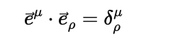
Given that the above Kronecker delta equals one when the indices are equal and zero when they are not equal, we know that it is a constant such that
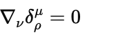
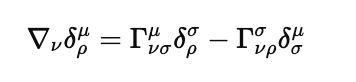
We can preserve this fact that the Kronecker delta delta derivative is zero, implying the constant value of the dot product of the covariant and contravariant basis vectors, only if the basis vectors themselves change in equal but opposite ways. The derivative of the Kronecker delta along coordinate v is composed of the derivative of the Kronecker delta component, and the derivative of both basis vectors using the product rule as shown below:

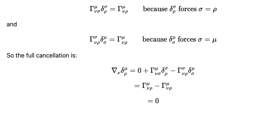
Because we know that the component never changes (it’s either always 1 or 0 ), we can simplify the above to:
which then equals 0, since
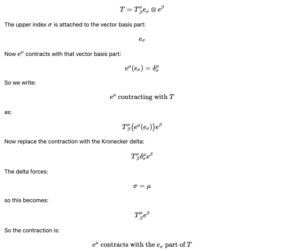
Now, when providing the derivative of any 1,1 tensor, we get the following:

The plus and minus terms containing the Christoffel symbol come from the facts above, namely that we must preserve the fact that
whose derivative across the v coordinate must be
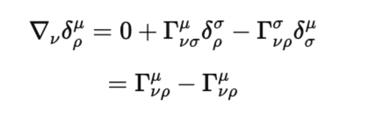
, so that when we take the product rule in differentiating tensor T across coordinate v, we get (remembering we have already implicitly multiplied by the dual basis eu and the basis vector ep):
Appendix 2: Geometrical Proof and Algebraic Poof of Isolating components of a mixed 1,1 Tensor
According to the diagram below, we have constructed vector A with covariant bases and contravariant components as well as with contravariant bases and covariant components. A1e1 is the contravariant component attached to the covariant base and A1e1 is the covariant component attached to contravariant base. Then, we must draw a right triangle with angle w is between the hypotenuse of vector A and a side parallel to e1, which we labeled D, and D perpendicular to the remaining side that we must draw in. We must then construct a second right triangle consisting of angle x between the hypotenuse of A1e1 and a constructed altitude perpendicular to side A2e2 . Note that while both of these two constructed right triangles are shown below to be part of a larger triangle, they do not have to be; it depends on the angles of the contravariant and covariant basis vectors).
In the bottom part of the page investigating how Ae1= A1 we must create a triangle with vector A as a hypotenuse, and then a side along basis vector e1 (in the diagram we labeled this side Q) that is perpendicular to a constructed height connecting to vector A. The angle that hypotenuse A makes with side Q is (x + w)
.
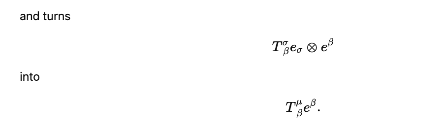
2. Isolating Components of a Mixed 1,1 Tensor: