The Metric Tensor and the Hidden Law of Cosines

The metric tensor is one of the most useful tools in mathematics. No matter your coordinate system, the metric tensor allows you to measure the same distances! However, for those unfamiliar with tensor calculus, the various subscripts and symbols of the metric tensor look like an indecipherable rune, and even for those who understand the symbols, the metric tensor may seem very abstract and divorced from the physical world. However, the metric tensor becomes much more tangible when it is seen as a crucial tool in relating any space to the very visualizable Law of Cosines. In order to show this deep connection, this post will proceed in the following way:

Prove the Law of Cosines, $\displaystyle c^2 = a^2 + b^2 - 2ab\cos(C)$ ;, for both acute and obtuse angles
Show how the Law of Cosines for Vectors, $\displaystyle |\vec{c}|^2 = |\vec{a}|^2 + |\vec{b}|^2 + 2\vec{a}\cdot\vec{b}$ intuitively applies to vector measurements,
Show how the Distance Invariant $\displaystyle ds^2 = g_{11}(dx^1)^2 + 2g_{12}dx^1dx^2 + g_{22}(dx^2)^2$ in tensor calculus uses the metric tensor to express the Law of Cosines for Vectors for flat space
Apply a more rigorous definition and deeper intuition of the metric tensor to see how the equivalence of the Distance Invariance to the Law of Cosines for Vectors is upheld in more complex spaces

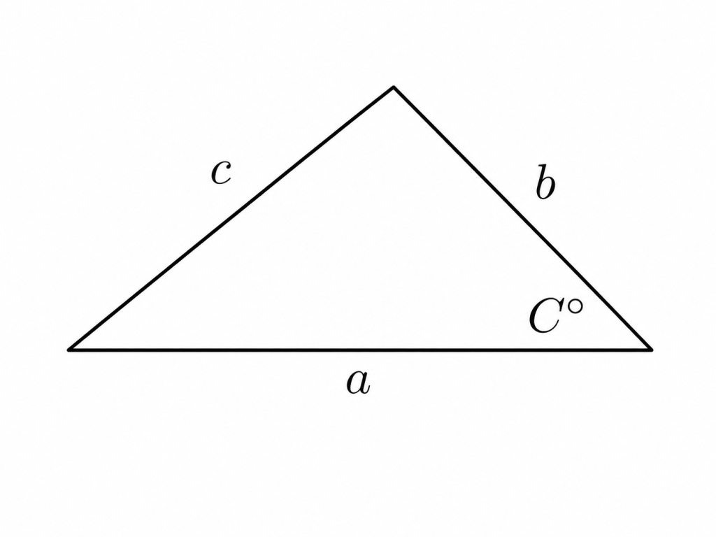
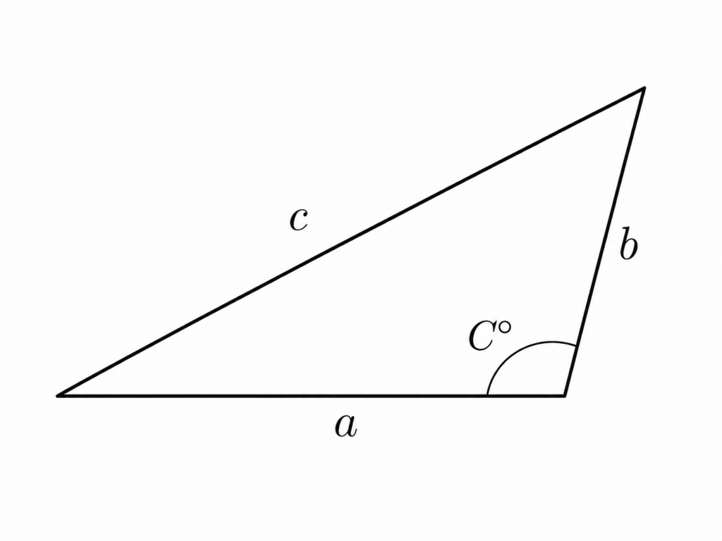
Proof of the Law of Cosines with an acute angle, given the triangle below. It is assumed we only know the values of sides a, b, and $\displaystyle \angle C^\circ$ .

First, draw the height of the triangle perpendicular to base a and label the right segment x and the left segment a-x:

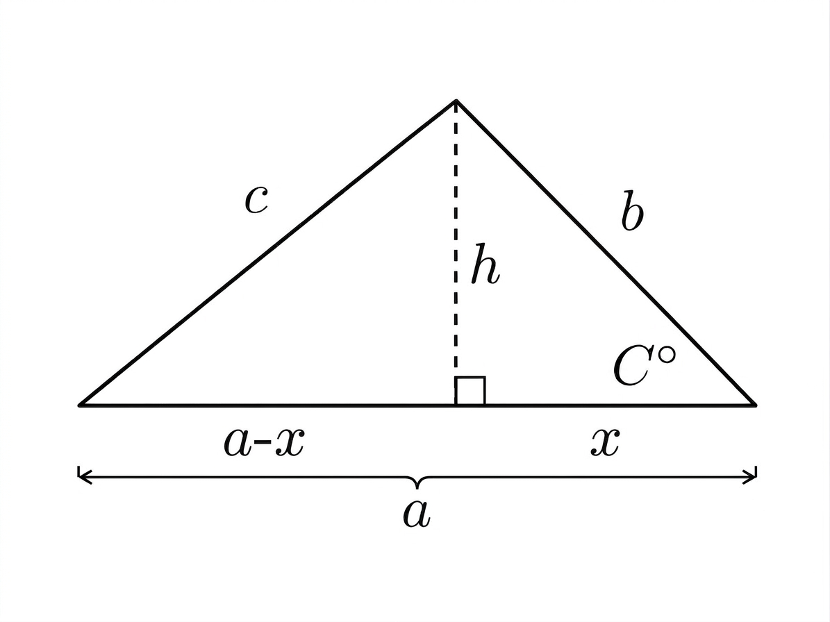
Now we see we have the following relationships:

$\displaystyle c^2 = h^2 + (a-x)^2$

with $\displaystyle h = b\sin(C), \qquad x = b\cos(C)$

Let’s plug these back into 1 to get:

2. $\displaystyle c^2 = \left(b\sin(C)\right)^2 + \left(a-b\cos(C)\right)^2$

Let’s expand the above :

3. $\displaystyle c^2 = \left(b\sin(C)\right)^2 + a^2 - 2ab\cos(C) + \left(b\cos(C)\right)^2$

Now group the 2 terms with the common factor b² and rearrange:

4. $\displaystyle c^2 = a^2 + b^2\left(\sin^2(C)+\cos^2(C)\right) - 2ab\cos(C)$

Plugging in $\displaystyle \sin^2(C)+\cos^2(C)=1$ to the above, we get

5. $\displaystyle c^2 = a^2 + b^2 - 2ab\cos(C)$

We see from the above picture that when angle C is acute, we effectively have side b of the triangle bend back towards side c, thereby diminishing the length of side c compared to a right triangle where b is perpendicular to a. This diminishing of the length of side c accounts for the negative sign in front of 2abcosC, which is a positive term when angle C is acute. So when angle C is acute, our Law of Cosines, $\displaystyle c^2 = a^2 + b^2 - 2ab\cos(C)$ , is saying, compared to constructing a right triangle whose squared hypotenuse length c is given by the Pythagorean Theorem c²= a² + b², we must subtract an additional 2abcosC term to account for the backward bending nature of side b and the consequent shortening of side c.

Let’s now prove the Law of Cosines for an obtuse angle:

Now let’s draw in a height h by extending base a by x and by labeling the angle supplementary to C as 180-C :

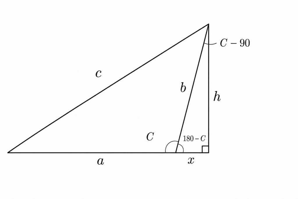
From the above picture it is clear that

$\displaystyle c^2 = (a+x)^2 + h^2$

with $\displaystyle x = b\cos(180^\circ-C)$ and $\displaystyle h = b\sin(180^\circ-C)$ . Plugging those 2 terms into equation 1, we get

2. $\displaystyle c^2 = \left(a+b\cos(180^\circ-C)\right)^2 + \left(b\sin(180^\circ-C)\right)^2$

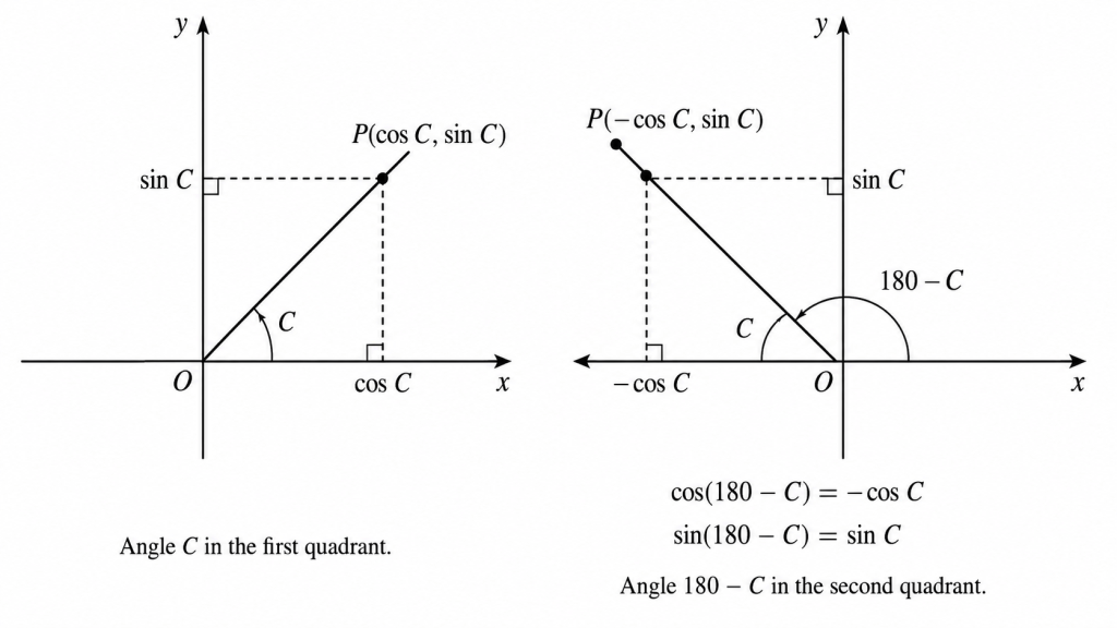
We can plug $\displaystyle \cos(180^\circ-C)=-\cos(C)$ and $\displaystyle \sin(180^\circ-C)=\sin(C)$ into equation 2. The picture below shows why we have these equalities:

After plugging these substitutions into equation 2. we now get:

3. $\displaystyle c^2 = \left(a - b\cos C\right)^2 + \left(b\sin C\right)^2$

Let’s expand the above to get

4. $\displaystyle c^2 = a^2 + b^2\left(\sin^2(C)+\cos^2(C)\right) - 2ab\cos(C)$

and substituting

$\displaystyle \sin^2(C)+\cos^2(C)=1$ back into 4. we get

5. $\displaystyle c^2 = a^2 + b^2 - 2ab\cos(C)$

When angle C is obtuse in our triangle, we effectively have side b bend further away from side c thereby comparatively elongating the length of side c. The cosine of an an obtuse angle, however, is negative, so the subtraction of -2abcosC when C is obtuse actually creates a positive term, showing that side c is longer than when angle C is acute. Compared to a right triangle formed by angle C equalling 90 degrees , when angle C is obtuse we find that c²is exactly -2abcosC greater than the Pythagorean Theorem’s c²= a² + b²

Of course, if angle C were 90 degrees, then cos(90)= 0, and our Law of Cosines, $\displaystyle c^2 = a^2 + b^2 - 2ab\cos(C)$ , reduces to the Pythagorean Theorem, c²= a² + b².

So we just derived and built some intuition for our Law of Cosines: $\displaystyle c^2 = a^2 + b^2 - 2ab\cos(C)$ ; now let’s understand this law when we are using vectors to form a triangle. We see that the Law of Cosines has a very similar form to our Law of Cosines for Vectors, $\displaystyle |\vec{c}|^2 = |\vec{a}|^2 + |\vec{b}|^2 + 2\vec{a}\cdot\vec{b}$ , as well as the Distance Invariant as measured by the metric tensor $\displaystyle ds^2 = g_{11}(dx^1)^2 + 2g_{12}dx^1dx^2 + g_{22}(dx^2)^2$ ; however, one big difference is that both the Law of Cosines for Vectors and the Distance Invariant as measured by the metric tensor are shown by addition signs, while the Law of Cosines has one subtraction sign. Let’s further explore this in the next section:

2. Law of Cosines Intuition Applied to Vector Measurement

We can derive a slightly different form of the law of cosines if we have vectors: $\displaystyle |\vec{c}|^2 = |\vec{a}|^2 + |\vec{b}|^2 + 2\vec{a}\cdot\vec{b}$ where the final term is the dot product between the two vectors, defined as $\displaystyle \vec{a}\cdot\vec{b} = |\vec{a}|\,|\vec{b}|\cos\theta$ . Note that the only big difference between the previously derived Law of Cosines and the Law of Cosines for Vectors is that the final term, the dot product of 2 vectors, is added rather than subtracted . Let’s get a better understanding of why this is so.

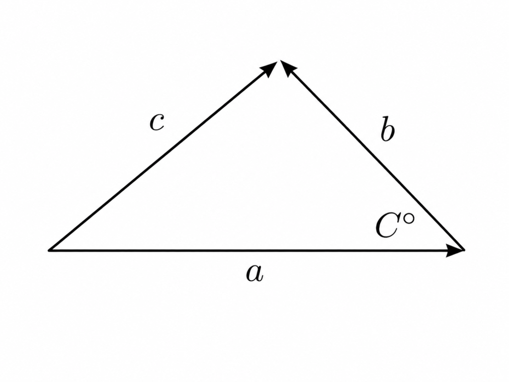
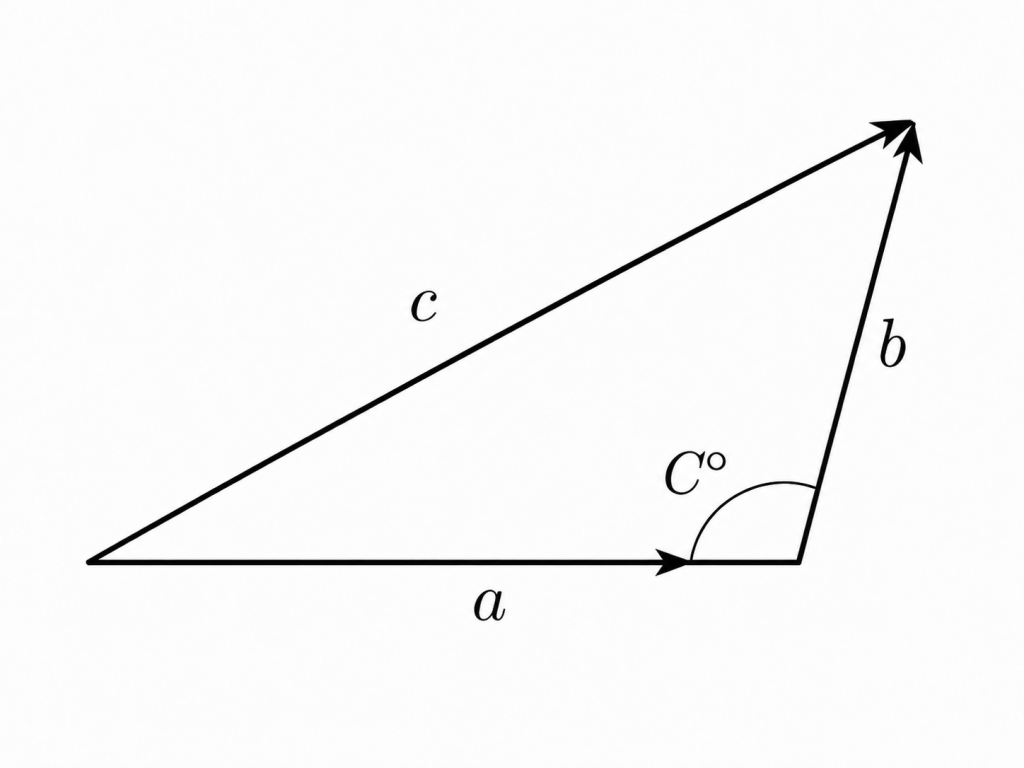
Below we have a triangle that shows the addition of two vectors $\displaystyle \vec{a}+\vec{b}=\vec{c}$ . Note that we must place vectors $\displaystyle \vec{a}+\vec{b}$ head to tail when we want to add them to sum to $\displaystyle \vec{c}$

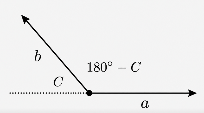
The final term in our original Law of Cosines, 2abcosC, is almost equivalent to twice the dot product of the vectors a and b. However, angle C as pictured above is no longer the relevant angle measurement for the vectors a and b; instead, when we take the dot product of two vectors, the tail of $\displaystyle \vec{a}$ must be attached to the tail of $\displaystyle \vec{b}$ ; in the above picture, we instead see that they are attached head-to-tail. In order to get the correct orientation of tail-to-tail we must translate $\displaystyle \vec{b}$ to the left so that its tail and the tail of $\displaystyle \vec{a}$ begin at the same point:

By taking the cosine of the angle between these tail-to-tail vectors, we correctly get the part of $\displaystyle \vec{b}$ that aligns with $\displaystyle \vec{a}$ and multiply this projection by $\displaystyle \vec{a}$ . We clearly see from the above that the relevant angle for the dot product, 180-C, is obtuse. When we take the cosine of an obtuse angle, we get a negative value, which correctly indicates how the projection of vector b points in the opposite direction of vector a. Additionally, because twice the dot product $\displaystyle 2ab\cos(180^\circ - C) = 2\vec{a}\cdot\vec{b}$ negative, the Law of Cosines for Vectors implies a shortening of vector C compared to a right triangle: $\displaystyle |\vec{c}|^2 = |\vec{a}|^2 + |\vec{b}|^2 + 2\vec{a}\cdot\vec{b}$ .

The dot product and its relevant angle of 180-C automatically account for the backward bending nature of vector b and the consequent shortening of vector c This, in fact, is the whole reason why we must place the vectors tail-to-tail; if we hadn’t, we would have calculated our dot product with the original acute angle of C, and therefore obtained a positive value for the dot product, which would have falsely indicated that the two vectors point in the same direction, implying that vector c would be elongated rather than shortened compared to a right triangle).

Thus, in the Law of Cosines for Vectors, we no longer need a negative sign in front of the dot product when angle C is acute; the angle formed by the tail-to-tail placement of the vectors, 180-C, already accounts for the backward bending direction that vector b makes to vector a and therefore embeds its own negative sign.

Let’s examine when $\displaystyle \angle C^\circ$ is obtuse, and 180-C is therefore acute, given the same vector lengths for a and b. Now, as shown below, vector b bends further away from vector c, thus giving vector c a longer distance to traverse, when compared to $\displaystyle \angle C^\circ$ being either acute or right:

In order to take the dot product of vectors a and b, lets translate vector b to the left so that it is tail-to-tail with vector a:

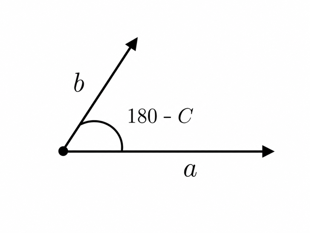
Now we see that 180-c is acute, so cos(180-c) is positive, which correctly indicates the fact that the projection of vector b points in the same direction as vector a. When C is obtuse, the dot product of $\displaystyle 2ab\cos(180^\circ - C) = 2\vec{a}\cdot\vec{b}$ is positive, so that the Law of Cosines for Vectors implies a lengthening of vector C compared to a right triangle: $\displaystyle |\vec{c}|^2 = |\vec{a}|^2 + |\vec{b}|^2 + 2\vec{a}\cdot\vec{b}$ . Note that the Law of Cosines for Vectors looks almost identical to the Distance Invariant provided by the metric tensor, $\displaystyle ds^2 = g_{11}(dx^1)^2 + 2g_{12}dx^1dx^2 + g_{22}(dx^2)^2$ ; now we just have to build our intuition for what the metric tensor and its funny notation actually mean.

3. The Distance Invariant as Measured by the Metric Tensor is the Law of Cosines

The metric tensor is an amazing mathematical tool that ensures that no matter the coordinates used, the distances calculated in any frame are always equivalent.

To understand what the metric tensor is, we must first define a few terms. As we already know, a vector is described by its components and directions. The component is a number that tells us how long the vector is in terms of a given coordinate basis direction. The direction, on the other hand, is given by a basis vector, which is defined by the coordinate system itself. Basis vectors are commonly written in the following notation: $\displaystyle \boxed{\vec{V} = V^\mu \mathbf{e}_\mu = V^\mu \frac{\partial}{\partial x^\mu}}$ , where $\displaystyle V^\mu \text{ are the contravariant components, while } \mathbf{e}_\mu \text{ are the basis vectors.}$ . The partial derivative $\displaystyle \frac{\partial}{\partial x^\mu}$ is a basis vector because it is assumed we apply it to the coordinate system itself, and when we do so, we always get a vector valued function of 1 coordinate unit in the chosen u direction and 0 in all the other directions (the metric tensor will help determine the basis vector’s actual physical length); thus, $\displaystyle \frac{\partial}{\partial x^\mu}$ is the same as $\displaystyle \vec{e}_u$

Now, in terms of the metric tensor, for two dimensions the distance measured in Cartesian coordinates is written as:

$\displaystyle ds^2 = g_{ij} \, dq^i dq^j, \qquad q^1 = x,\quad q^2 = y,\quad dq^1 = dx,\quad dq^2 = dy$ , and g_ij equaling the dot products of the relevant basis vectors: $\displaystyle g_{ij}=\mathbf{e}_i\cdot\mathbf{e}_j$

The above can be expanded according to the Einstein Summation convention (the Einstein summation convention means that when an index appears twice in one term, once as an upper index and once as a lower index, you automatically sum over that index.) to the more familiar $\displaystyle ds^2 = g_{11}(dq^1)^2 + 2g_{12}dq^1dq^2 + g_{22}(dq^2)^2$ .

Let’s see how the Distance Invariant with the Metric Tensor is equivalent to the Law of Cosines in the simplest cases. Below are the basis vectors of coordinate length 1 in the Cartesian coordinate system:

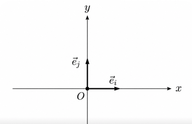
And here is a vector, composed of components and basis vectors:

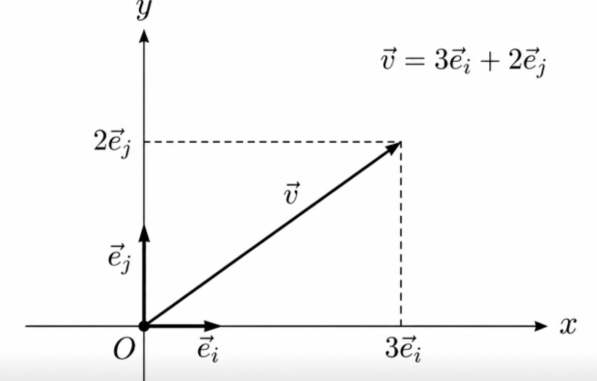
Now the metric tensor stores the dot products of all the combinations of the basis vectors of a coordinate system. With an angle of 90 between basis vectors and their lengths as 1, our metric tensor is:

$\displaystyle g = \left( \begin{array}{cc} \vec e_i \cdot \vec e_i & \vec e_i \cdot \vec e_j \cr \vec e_j \cdot \vec e_i & \vec e_j \cdot \vec e_j \end{array} \right) = \left( \begin{array}{cc} \vec e_1 \cdot \vec e_1 & \vec e_1 \cdot \vec e_2 \cr \vec e_2 \cdot \vec e_1 & \vec e_2 \cdot \vec e_2 \end{array} \right) = \left( \begin{array}{cc} 1 & 0 \cr 0 & 1 \end{array} \right)$

Given the values our vector components, we get the following for the square of the distance:

$\displaystyle ds^2 = g_{ij}\,dq^i dq^j = g_{11}(dq^1)^2 + 2g_{12}dq^1dq^2 + g_{22}(dq^2)^2 = 1(3)^2 + 2(0)(3)(2) + 1(2)^2 = 9+4 = 13$ .

Notice this is exactly the same value for what the Law of Cosines for Vectors would give:

$\displaystyle |\vec c|^2 = |\vec a+\vec b|^2 = \vec a\cdot \vec a + 2\vec a\cdot \vec b + \vec b\cdot \vec b = |\vec a|^2 + 2|\vec a||\vec b|\cos\theta + |\vec b|^2 = 3^2 + 2(3)(2)\cos 90^\circ + 2^2 = 9 + 0 + 4 = 13$

which is of course the same as what our original Law of Cosines for Triangles gives (note that theta is still 90 degrees, since 180-90=90:

$\displaystyle |\vec c|^2 = |\vec a|^2 + |\vec b|^2 - 2|\vec a||\vec b|\cos\theta = 3^2 + 2^2 - 2(3)(2)\cos 90^\circ = 9 + 4 - 12(0) = 13$

Now let’s see what happens if the basis vectors aren’t perpendicular, but rather are separated by a head-to-tail angle of 120 degrees, which corresponds to a tail-to-tail angle of 60 degrees. Compared to when the angle was 90 degrees, the distance measured is greater in both the Law of Cosines for Vectors and the Distance Invariant with the Metric Tensor:

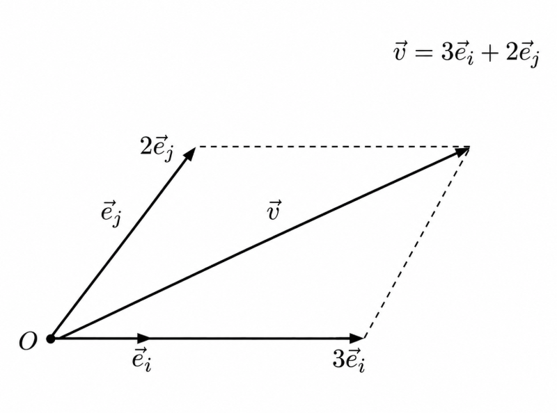
Our metric tensor now becomes $\displaystyle g = \left( \begin{array}{cc} \vec e_1 \cdot \vec e_1 & \vec e_1 \cdot \vec e_2 \cr \vec e_2 \cdot \vec e_1 & \vec e_2 \cdot \vec e_2 \end{array} \right) = \left( \begin{array}{cc} 1 & \cos 60^\circ \cr \cos 60^\circ & 1 \end{array} \right) = \left( \begin{array}{cc} 1 & \frac{1}{2} \cr \frac{1}{2} & 1 \end{array} \right)$

so our distance invariant using the metric tensor is

$\displaystyle ds^2 = g_{ij}\,dq^i dq^j = g_{11}(dq^1)^2 + 2g_{12}dq^1dq^2 + g_{22}(dq^2)^2 = 1(3)^2 + 2\left(\frac{1}{2}\right)(3)(2) + 1(2)^2 = 9+6+4 = 19$

and our Law of Cosines for Vectors gets the same distance:

$\displaystyle |\vec c|^2 = |\vec a + \vec b|^2 = \vec a \cdot \vec a + 2\vec a \cdot \vec b + \vec b \cdot \vec b = |\vec a|^2 + 2|\vec a||\vec b|\cos\theta + |\vec b|^2 = 3^2 + 2(3)(2)\cos(180^\circ - 120^\circ) + 2^2 = 9 + 12\left(\frac{1}{2}\right) + 4 = 19$ .

and it is also the same for our original Law of Cosines for triangles, noting that now theta is 120 degrees instead of 60:

$\displaystyle |\vec c|^2 = |\vec a|^2 + |\vec b|^2 - 2|\vec a||\vec b|\cos(\theta) = 3^2 + 2^2 - 2(3)(2)\cos(120^\circ) = 9 + 4 - 12\left(-\frac{1}{2}\right) = 19$

4. A Deep Dive into the Metric Tensor Intuition and the Application of the Distance Invariant and Law of Cosines to More Complex Spaces

So far, we have seen that the metric tensor acts like a local Law of Cosines inside one coordinate system. Now we will see its deeper power: it changes from coordinate system to coordinate system in exactly the way needed to keep $ds^2$ the same.

The true magic of the metric tensor is the fact that $\displaystyle ds^2 = g_{ij}\,dq^i dq^j = g'_{\alpha\beta}\,dq'^\alpha dq'^\beta$ , which says that no matter your coordinate system, the distance measured must be the same! Why must our measured distance be the same no matter which basis vectors are used?

It all has to do with how we convert between different coordinate systems, and then the metric tensor stores that knowledge for the purpose of measuring distances. The coordinate transformation tells us how the new basis vectors are built from the old basis vectors. Once we know how these new basis vectors are built from the original basis vectors, the metric tensor records the new basis vectors’ dot products in terms of the original basis vectors. Then, the metric tensor organizes this information in a way that makes distance calculations very easy.

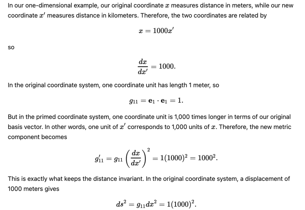
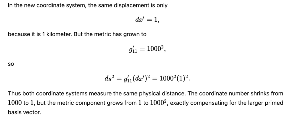
As a very simple, concrete example, imagine you have a basis vector of 1 meter pointing east, and you measure a distance of 1000 meters. Then, we rescale the basis vector so that it is now 1,000 times bigger; this new basis vector now represents 1 kilometer in a new coordinate system. What happens to our distance when we measure it in this new coordinate system? We now record 1 km of distance; this means that while we expanded the size of the basis vector by 1000, we shrunk the size of vector component by 1/1000, as in the following picture:

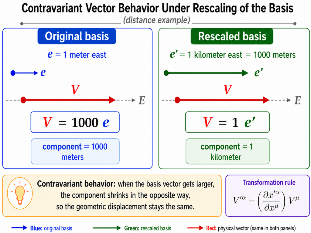
So while one person records 1000m with the 1 meter due East basis vector, the other person records 1km with the 1 km due East basis vector, but we are talking about the same physical distance vector with the same distance traversed (just in different units). The metric tensor helps to convert our new coordinate system into the terms of the old coordinate system by first relying on the relationship between the coordinates:

The previous example was the simplest possible. But what if the basis vectors are not only different lengths but also different angles to each other like when our original basis vectors are Cartesian and our new coordinate system has polar basis vectors:

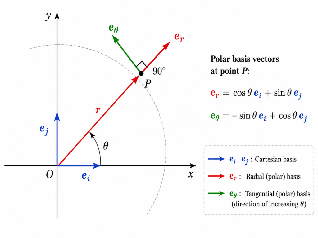
In terms of polar coordinates, our Cartesian coordinates are: $\displaystyle x=r\cos\theta,\qquad y=r\sin\theta$

Now we must figure out how our polar basis vectors are built from our Cartesian basis vectors, using Einstein Summation Convention: $\displaystyle \mathbf e'_{\alpha}=\frac{\partial q^i}{\partial q^{\prime\alpha}}\mathbf e_i$ .

In building our new polar basis vectors out of each of the old Cartesian basis vectors, we get the following:

$\displaystyle \mathbf e'_r=\frac{\partial x}{\partial r}\mathbf e_i+\frac{\partial y}{\partial r}\mathbf e_j=\cos\theta\,\mathbf e_i+\sin\theta\,\mathbf e_j$ and $\displaystyle \mathbf e'_{\theta}=\frac{\partial x}{\partial \theta}\mathbf e_i+\frac{\partial y}{\partial \theta}\mathbf e_j=-r\sin\theta\,\mathbf e_i+r\cos\theta\,\mathbf e_j$

Below in the top of the diagram, I added how this transform of $\displaystyle \mathbf e'_{\alpha}=\frac{\partial q^i}{\partial q^{\prime\alpha}}\mathbf e_i$ .is geometrically accomplished through the mapping of the original basis vectors onto the new basis vectors:

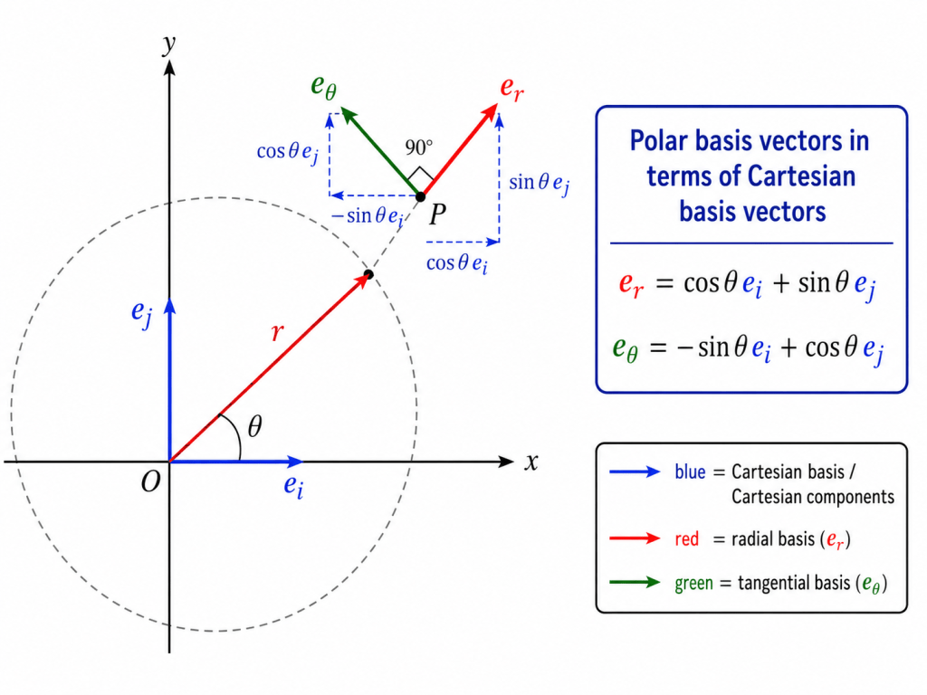
So, we literally see how each polar basis vector is built from various combinations of our Cartesian basis vectors.

Now that we have solved for our Polar basis vectors in terms of our Cartesian basis vectors, we can take the dot products as in the following to get the polar metric:

The general distance invariant in terms of our primed coordinates is $\displaystyle ds^2 = g_{rr}^{\prime}(dr)^2 + g_{r\theta}^{\prime}\,dr\,d\theta + g_{\theta r}^{\prime}\,d\theta\,dr + g_{\theta\theta}^{\prime}(d\theta)^2$ , which equals

$\displaystyle ds^2 = g_{rr}^{\prime}(dr)^2 + 2g_{r\theta}^{\prime}\,dr\,d\theta + g_{\theta\theta}^{\prime}(d\theta)^2$ , so when we fill in our polar metric we get

$\displaystyle ds^2 = 1(dr)^2 + 2(0)\,dr\,d\theta + r^2(d\theta)^2$ , which simplifies to $\displaystyle ds^2=dr^2+r^2d\theta^2$

This tells us that the distance measured when using polar coordinates is:: $\displaystyle ds^2=dr^2+r^2d\theta^2$ . The coefficient in front of dr² is 1, showing us that measuring 1 unit of length in dr would be equivalent to 1 unit of length in the Cartesian coordinate system. However, the coefficient in front of $\displaystyle \theta^2$ is r², showing that our basis vectors along $\displaystyle \theta$ actually get longer by a factor of r as r increases, This matches our expectation, since the distance measured around an arc is equal to r $\displaystyle \theta$ , when $\displaystyle \theta$ is measured in radians. For example, when r is 1, 1 radian of $\displaystyle \theta$ corresponds to 1 unit of length in our Cartesian system , but when r=5, 1 radian of $\displaystyle \theta$ corresponds to 5 units of length in our Cartesian system.

The distance invariant for the polar metric, $\displaystyle ds^2=dr^2+r^2d\theta^2$ , is the Law of Cosines for Vectors in disguise. We most clearly see that relationship in the previously highlighted step of $\displaystyle ds^2 = g_{rr}^{\prime}(dr)^2 + 2g_{r\theta}^{\prime}\,dr\,d\theta + g_{\theta\theta}^{\prime}(d\theta)^2$ which exactly matches the Law of Cosines for Vectors. Therefore, the distance invariant for the polar metric is saying: if we track the polar basis vectors in terms of our Cartesian basis vectors and then take their dot products (these are all of our g’ terms), we can use the Law of Cosines for Vectors to measure the distance traveled by changes in the polar coordinates, $\displaystyle dr$ and $\displaystyle d\theta$ , in terms of our original Cartesian coordinate system!

So far we have learned the following:

That the Law of Cosines and the Distance Invariant using the Metric Tensor measure distances by taking into account both angles and lengths of the coordinate bases in the same general formula using the same geometric ideas.
That the Distance Invariant using the Metric Tensor can also translate between different coordinate systems in order to arrive at the distance measured by a chosen original coordinate frame, in our case Cartesian.

What we haven’t given an intuition to yet is:

Can the Distance Invariant using the Metric Tensor still be equal to the Law of Cosines for curved spaces, not just flat spaces?
How can we visualize applying the Law of Cosines to Higher Dimensional spaces?

Let’s address the first of these points now: can the Distance Invariant using the Metric Tensor still be equal to the Law of cosines for curved spaces, specifically the surface of a sphere. Though we will start with three dimensions to explore spherical coordinates, we will end up restricting the following example to 2 dimensions to better understand how the Law of Cosines emerges even on a curved surface:

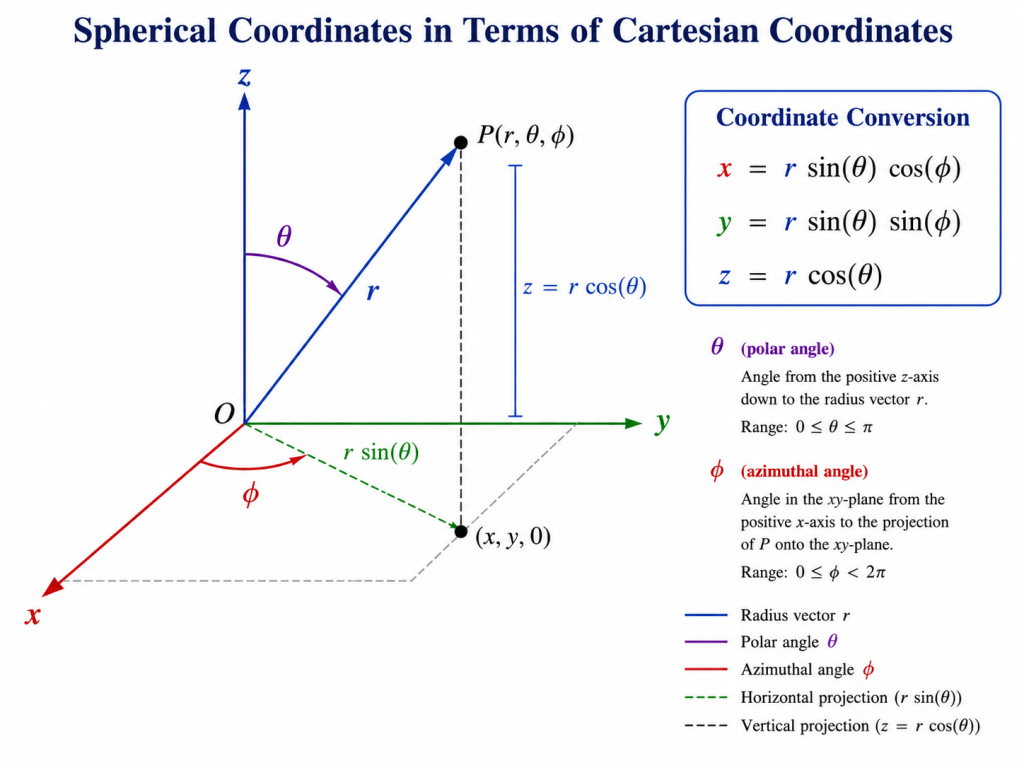
Taking all of our partial derivatives we get:

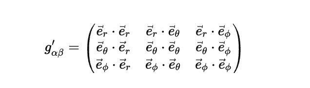
$\displaystyle \frac{\partial(x,y,z)}{\partial(r,\theta,\phi)} = \left( \begin{array}{ccc} \frac{\partial x}{\partial r} & \frac{\partial x}{\partial \theta} & \frac{\partial x}{\partial \phi} \cr \frac{\partial y}{\partial r} & \frac{\partial y}{\partial \theta} & \frac{\partial y}{\partial \phi} \cr \frac{\partial z}{\partial r} & \frac{\partial z}{\partial \theta} & \frac{\partial z}{\partial \phi} \end{array} \right) = \left( \begin{array}{ccc} \sin\theta\cos\phi & r\cos\theta\cos\phi & -r\sin\theta\sin\phi \cr \sin\theta\sin\phi & r\cos\theta\sin\phi & r\sin\theta\cos\phi \cr \cos\theta & -r\sin\theta & 0 \end{array} \right)$

Because $\displaystyle \vec e_{\alpha}^{\prime}=\frac{\partial x^i}{\partial q^{\alpha}}\hat e_i$ , e_r is calculated as $\displaystyle \vec e_r=\frac{\partial x^i}{\partial r}\hat e_i$ , so after plugging in the relevant partial derivatives in from the above matrix with dr as the denominator, we get that, in terms of our Cartesian coordinate bases, $\displaystyle \vec e_r=(\sin\theta\cos\phi)\hat x+(\sin\theta\sin\phi)\hat y+(\cos\theta)\hat z$ . In terms of our Cartesian coordinate bases, our other spherical coordinate bases become $\displaystyle \vec e_\theta=(r\cos\theta\cos\phi)\hat x+(r\cos\theta\sin\phi)\hat y+(-r\sin\theta)\hat z$ and $\displaystyle \vec e_\phi=\left(-r\sin\theta\sin\phi,r\sin\theta\cos\phi,0\right)$ . Plugging these values into the metric tensor matrix of

we get (please zoom in on the matrix below to see all the terms written out more legibly)

After simplifying each dot product we get:

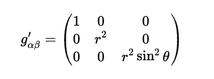
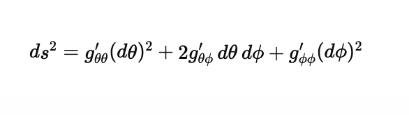
So our spherical distance formula is

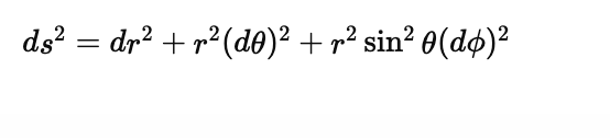
If we restrict ourselves to being on the surface of a sphere with constant radius length r, our dr term is 0 since we are not moving radially and we get the spherical distance formula of $\displaystyle ds^2=r^2(d\theta)^2+r^2\sin^2\theta(d\phi)^2$ , which like our other worked examples is 2 dimensional. Note that thus far, we have used the exact same process in converting between the Cartesian 2-d coordinates and the Spherical surface 2-d coordinates as we did when we converted between the Cartesian 2-d coordinates and the Polar 2-d coordinates. To see exactly why this is true by reverse engineering back to the Law of Cosines for Vectors: for the 2-d sphere, we derived $\displaystyle ds^2=r^2(d\theta)^2+r^2\sin^2\theta(d\phi)^2$ , which is built from the full metric components in $\displaystyle ds^2=r^2(d\theta)^2+2(0)\,d\theta\,d\phi+r^2\sin^2\theta(d\phi)^2$ , which we plugged in according to the general formula of:

which, as previously discussed, is equivalent to the Law of Vectors for Cosines.

Note that this final expression gives the dot products of spherical surface basis vectors in terms of our Cartesian basis vectors (these are all of our g’ terms), and then uses the Law of Cosines for Vectors to calculate the distance traversed on our spherical surface.

Though this distance invariant for the surface of a sphere, $\displaystyle ds^2=r^2(d\theta)^2+r^2\sin^2\theta(d\phi)^2$ , really uses the Law of Cosines to measure the distance traveled by the spherical coordinate changes, we must add one important caveat: the coordinate changes on the spherical surface must be infinitesimal, as implied by our partial derivatives (which track infinitesimal changes), in order to maintain the equality between the Law of Cosines and the Distance Invariant Measured by the Metric Tensor on a sphere. The reason why the spherical surface changes must be infinitesimal is because over longer distances on a sphere, ordinary straight lines break down and instead straight lines are curved geodesics. However, we can still measure longer distances on a spherical surface by taking the integral of ds after we solve for ds in the expression $\displaystyle ds^2=r^2(d\theta)^2+r^2\sin^2\theta(d\phi)^2$ ; by taking the integral of ds, we essentially add up all the infinitesimal distances traversed as measured by the local Law of Cosines, shown by the following expression $\displaystyle s=\int ds=\int r\sqrt{(d\theta)^2+\sin^2\theta(d\phi)^2}$ . There are two profound implications of this: firstly, that if we traverse an infinitesimal distance in a curved, or generally non-flat, space, it is always locally flat and thus suitable for the Law of Cosines embedded in the Distance Invariant using the Metric Tensor expression. Secondly, that we can calculate arbitrarily longer distances in non-flat space using the integral sums of the infinitesimal distances calculated by the Law of Cosines embedded in the Distance Invariant using the Metric Tensor expression.

Now that we have shown that the distances in non-flat space are still calculable from the Law of Cosines embedded in the Distance Invariant, let’s address our final point: understanding how the Law of Cosines and the Distance Invariant apply to higher dimensions. If we have a 3 dimensional vector, with basis vectors e₁, e₂ and e₃ along with corresponding components a, b and c, then the Law of Cosines for Vectors is:

If the basis vectors are perpendicular in such a space, all the cosine terms go to 0 and we get the Pythagorean Theorem for three dimesnions. However, let’s present a case where none of the basis vectors are perpendicular to make it slightly more interesting:

In the image below, we would like to calculate the length of the vector composed of ae₁ + be₂ + ce₃

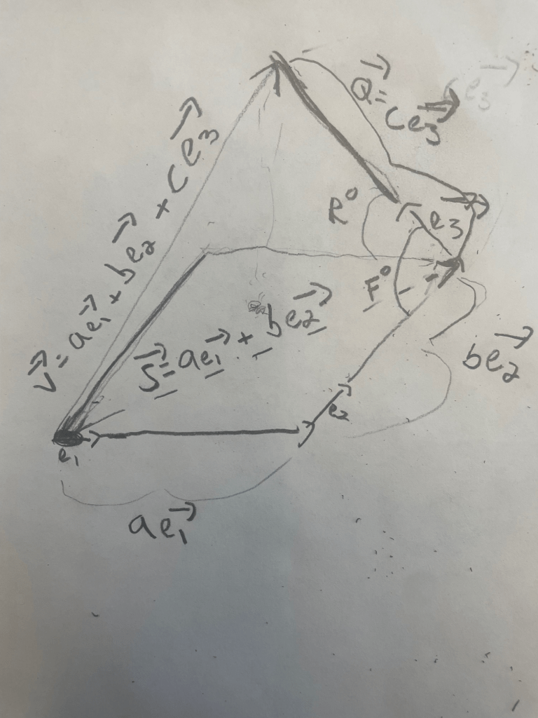
We see that vector v is composed of 3 vectors with 3 bases (namely ae₁, be₂ and ce₃), but we can simplify the problem by thinking of vector v being composed of only 2 vectors, vectors S and Q. By simplifying, we can now easily use the Vector Law of Cosines with vectors S and Q to calculate the length of vector v: $\displaystyle v^2=S^2+Q^2+2\vec{S}\cdot\vec{Q}$ . Because vector S is made up of two basis vectors e₁ and e₂ the single basis vector belonging to vector Q, e₃, makes 2 separate angles with each of these 2 separate basis vectors, namely angles R and F. Luckily, dot products make it very easy to calculate these separate angles.

Before we explore the dot products, let’s first break vector S down with the Vector Law of Cosines: $\displaystyle S^2=\left(a\mathbf{e}_1\right)^2+\left(b\mathbf{e}_2\right)^2+2ab\,\mathbf{e}_1\cdot\mathbf{e}_2$

Substituting $\displaystyle S^2=\left(a\mathbf{e}_1\right)^2+\left(b\mathbf{e}_2\right)^2+2ab\,\mathbf{e}_1\cdot\mathbf{e}_2$ back into $\displaystyle v^2=S^2+Q^2+2\vec{S}\cdot\vec{Q}$ , we get

$\displaystyle V^2=\left(a\mathbf{e}_1\right)^2+\left(b\mathbf{e}_2\right)^2+2ab\,\mathbf{e}_1\cdot\mathbf{e}_2+Q^2+2\vec{S}\cdot\vec{Q}$

Now Q² is just (ce₃)², so upon substitution our previous equation becomes $\displaystyle V^2=\left(a\mathbf{e}_1\right)^2+\left(b\mathbf{e}_2\right)^2+2ab\,\mathbf{e}_1\cdot\mathbf{e}_2+\left(c\mathbf{e}_3\right)^2+2\vec{S}\cdot\vec{Q}$ .

The final step is to get the dot product of S and Q in terms of our basis vectors, so now we must break down vector S into the two bases it is composed of, e₁and e₂, and express vector Q in terms of its basis e₃:

2 $\displaystyle \vec{S}\cdot \vec{Q}$ = $\displaystyle 2(a\mathbf{e}_1+b\mathbf{e}_2)\cdot c\mathbf{e}_3=2ac\,\mathbf{e}_1\cdot\mathbf{e}_3+2bc\,\mathbf{e}_2\cdot\mathbf{e}_3$

Substituting this expression for 2 $\displaystyle \vec{S}\cdot \vec{Q}$ into $\displaystyle V^2=\left(a\mathbf{e}_1\right)^2+\left(b\mathbf{e}_2\right)^2+2ab\,\mathbf{e}_1\cdot\mathbf{e}_2+\left(c\mathbf{e}_3\right)^2+2\vec{S}\cdot\vec{Q}$

we finally get:

$\displaystyle V^2=\left(a\mathbf{e}_1\right)^2+\left(b\mathbf{e}_2\right)^2+2ab\,\mathbf{e}_1\cdot\mathbf{e}_2+\left(c\mathbf{e}_3\right)^2+2ac\,\mathbf{e}_1\cdot\mathbf{e}_3+2bc\,\mathbf{e}_2\cdot\mathbf{e}_3$

Now if we were to use the Distance Invariant with the metric tensor, we would have

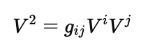
which upon expanding using our specific vector components would become:

$\displaystyle V^2=a^2g_{11}+b^2g_{22}+c^2g_{33}+2abg_{12}+2acg_{13}+2bcg_{23}$ , and then plugging in our specific basis vectors arrives at the exact same equation:

$\displaystyle V^2=a^2(\mathbf{e}_1\cdot\mathbf{e}_1)+b^2(\mathbf{e}_2\cdot\mathbf{e}_2)+c^2(\mathbf{e}_3\cdot\mathbf{e}_3)+2ab(\mathbf{e}_1\cdot\mathbf{e}_2)+2ac(\mathbf{e}_1\cdot\mathbf{e}_3)+2bc(\mathbf{e}_2\cdot\mathbf{e}_3)$ . This is exactly the same equation as what we derived using our Vector Law of Cosines!

What about if we had even more dimensions? The distance invariant would still take the same form. To see why with an example of a 4 dimensional vector, we can assume it is composed of 2 separate vectors to simplify the problem, just as we did with the 3 dimensional vector v in our previous example. Let’s assume that this new 4 dimensional vector, called vector z, can be broken down into the 3 dimensional vector v and then an additional dimension spanned by vector f. Then the Vector Law of Cosines gives:

$\displaystyle |\vec{z}|^2=|\vec{v}|^2+|\vec{f}|^2+2\vec{v}\cdot\vec{f}$

We can plug in $\displaystyle V^2=\left(a\mathbf{e}_1\right)^2+\left(b\mathbf{e}_2\right)^2+\left(c\mathbf{e}_3\right)^2+2ab\,\mathbf{e}_1\cdot\mathbf{e}_2+2ac\,\mathbf{e}_1\cdot\mathbf{e}_3+2bc\,\mathbf{e}_2\cdot\mathbf{e}_3$ to get

$\displaystyle |\vec{z}|^2=\left(a\mathbf{e}_1\right)^2+\left(b\mathbf{e}_2\right)^2+\left(c\mathbf{e}_3\right)^2+2ab\,\mathbf{e}_1\cdot\mathbf{e}_2+2ac\,\mathbf{e}_1\cdot\mathbf{e}_3+2bc\,\mathbf{e}_2\cdot\mathbf{e}_3+|\vec{f}|^2+2(a\mathbf{e}_1+b\mathbf{e}_2+c\mathbf{e}_3)\cdot\vec{f}$

Now let’s assume vector f has component d with basis vector e₄. We can plug that in to the above expression to obtain

$\displaystyle |\vec{z}|^2=\left(a\mathbf{e}_1\right)^2+\left(b\mathbf{e}_2\right)^2+\left(c\mathbf{e}_3\right)^2+2ab\,\mathbf{e}_1\cdot\mathbf{e}_2+2ac\,\mathbf{e}_1\cdot\mathbf{e}_3+2bc\,\mathbf{e}_2\cdot\mathbf{e}_3+\left(d\mathbf{e}_4\right)^2+2(a\mathbf{e}_1+b\mathbf{e}_2+c\mathbf{e}_3)\cdot d\mathbf{e}_4$

which upon rearranging terms and expanding the dot product gives:

$\displaystyle |\vec{z}|^2=\left(a\mathbf{e}_1\right)^2+\left(b\mathbf{e}_2\right)^2+\left(c\mathbf{e}_3\right)^2+\left(d\mathbf{e}_4\right)^2+2ab\,\mathbf{e}_1\cdot\mathbf{e}_2+2ac\,\mathbf{e}_1\cdot\mathbf{e}_3+2bc\,\mathbf{e}_2\cdot\mathbf{e}_3+2ad\,\mathbf{e}_1\cdot\mathbf{e}_4+2bd\,\mathbf{e}_2\cdot\mathbf{e}_4+2cd\,\mathbf{e}_3\cdot\mathbf{e}_4$

Of course, the distance invariant with the metric tensor would give the equivalent expression:

$\displaystyle |\vec{z}|^2=a^2g_{11}+b^2g_{22}+c^2g_{33}+d^2g_{44}+2abg_{12}+2acg_{13}+2adg_{14}+2bcg_{23}+2bdg_{24}+2cdg_{34}$

We can continue this iterative process for as many dimensions as we would like using the same repetition:

Compose an n dimensional vector out of 2 separate vectors, an n-1 dimensional vector and a 1 dimensional vector (which is the nth dimension newly added).
Take the Law of Cosines for Vectors using the n-1 dimensional vector and the 1 dimensional vector
Plug in the Law of Cosines expression that already measured the length of the n-1 dimensional vector into the equation in step 2.
Plug in the vector basis and component of the 1 dimension vector into the equation in step 2.
Now, with these substituted terms, expand twice the dot product of the 1 dimensional vector with each separate basis of the previous n-1 dimensional vector, and rearrange terms

The Law of Cosines turns out to be more profound than when I first encountered it in 9th grade geometry. Though the Law of Cosines takes different forms for triangles, vectors and the Distance Invariant in tensor calculus, it ultimately is the foundation for each. We also showed in this post what makes the metric tensor unique: that it allows us to convert our distances seamlessly from one coordinate frame to another, no matter if the space is flat or curved. But underlying the complicated notation of the Distance Invariant with the Metric Tensor is ultimately the Law of Cosines! Not only does the Law of Cosines underlie calculations of distance for both flat and curved spaces, but it also is used to measure distances in any dimensional space that we so choose. This powerful yet simple geometric law is often hidden behind complex notation, but when we dig deep enough, we rediscover its importance.

The Metric Tensor and the Hidden Law of Cosines

Published by Josh Fialkow

Leave a comment Cancel reply

Share this:

Related

Published by Josh Fialkow

Leave a comment Cancel reply