Perimeter Growth versus Area Loss: The Race that Determines Fractal Dimensions of Coastlines

This post is about how an entire geological story can be embedded in a single number, a number that weaves together the degree of volcanic activity, rock type, river flow, sea level rise and presence of coral reefs, amongst other influences. And from the implications of this number in the geological story, we can derive general principles that apply to biology too. This special kind of number is the fractal dimension, used to measure a fractal shape, which is defined as a shape with meaningful detail at every scale, so zooming in reveals new structure rather than a smooth edge. Many patterns in nature exhibit fractal-like behavior over a variety of scales: for example, a few famous fractal patterns include cloud perimeters, river networks, tree branching, and coastlines. We will focus on the last of these- the fractal quality of coastlines- to help us understand the unique stories of a few islands in one of my favorite places in the world: the Caribbean. We will also derive a new way to understand fractal dimension in terms of a race between two dimensions.

To first understand what a fractal is (for video reference, please visit 3 Blue, 1 Brown’s video https://www.youtube.com/watch?v=gB9n2gHsHN4 for the best introduction to understanding fractals), we must define the concept of dimension in an intuitive fashion.

Let’s start with the first dimension: a line is one dimensional because it has a single axis of measurement, let’s call it the x-axis, and only needs a single number to describe a point’s location along that axis. A piece of paper is two dimensional because it has two axes of measurement, the x-axis and y-axis, and needs two numbers to describe a point’s location in that space. Our spatial world is three dimensional because we have 3 axes to describe location: x, y and z. On the other hand, a single point of infinitesimal size is 0 dimensional, since there is no number necessary to describe where you are on the point (if on the point, you can only be on the point and not anywhere else). But is there any room for dimensions between 0 and 1 or 1 and 2? Can we properly think of a dimensionality of 1.2? The fractal dimension is the answer to our dimensional dilemma.

There are different ways to define fractal dimension, but we will mainly use two. The first definition relates a shape’s “mass” to how it scales. By “mass,” we mean the number of self-similar copies needed to rebuild the original shape, where each copy is just a smaller version of the whole. For instance, a square of side length 1 can be reconstructed from 4 smaller squares, each with side length 1/2. Thus, when the length scale is reduced by a factor of $1/2$, the number of self-similar copies is 4 (it would take 4 copies of s=1/2 to rebuild the original square).

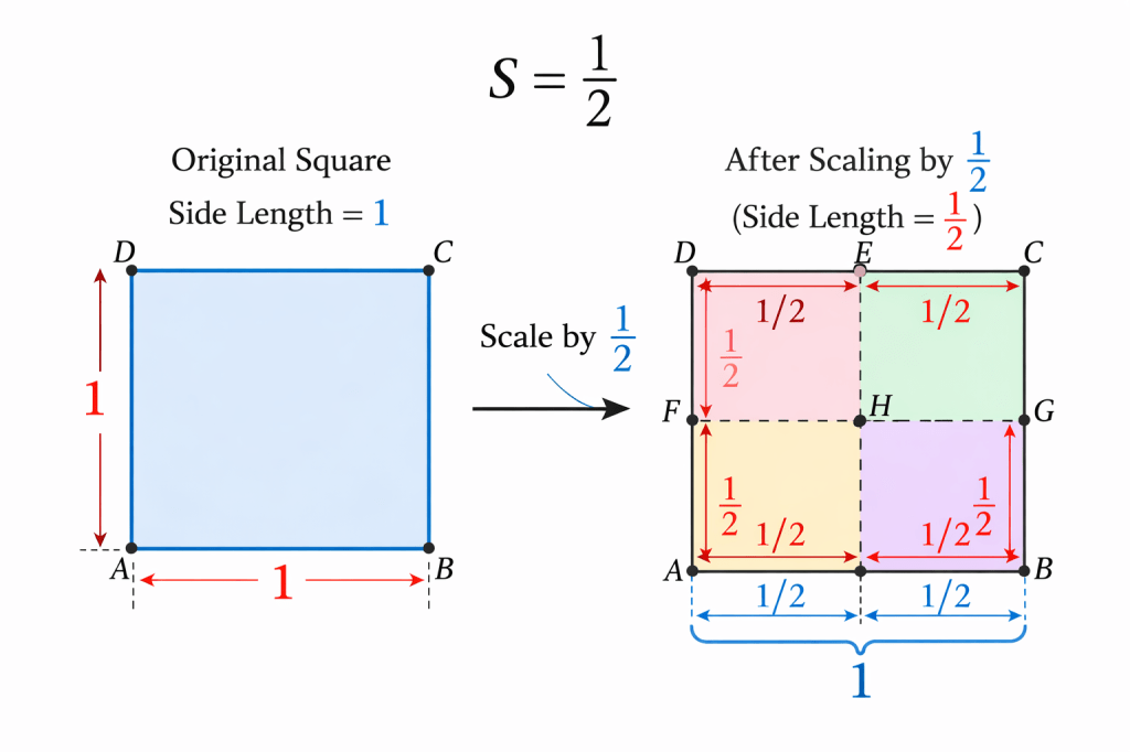
We can relate the mass, or number of self-similar copies, and the scale factor s by raising s factor to the power -d, as in:

Using our previous example where the mass of the figure is 4 after scaling by 1/2, our equation would become

where d=2. This exponent d is actually the dimension! A square, as we know, has two dimensions, which checks out with the previous equation. If we had scaled the square by a factor of 1/3, its mass would have increased to 9 (we would get 9 self similar copies of s=1/3 to get the original square), as in where d still equals two. So no matter the scale factor, the mass of a figure of a certain dimension will always increase according to . Note that a square is not a fractal because its local geometry stabilizes under magnification: away from the corners it converges to a straight line, and at the corners it converges to a fixed angle and then doesn’t change at all. A fractal, by contrast, exhibits different structure at arbitrarily small scales. Thus, we know a shape is not a fractal if, by zooming in, the shape no longer reveals new structure, whereas with a fractal, magnification never settles into an unchanging, stable form.

If we continued this process of scaling the square by 1/2 in multiple iterations, for any given iteration for our square our equation for fractal dimension would become , where the ratio of M_n+1:M_n would always be 4 given that d always equals 2; if our s=1/3, then that same ratio would always be 9, given that d=2.

Now let’s examine the properties of a true fractal, the Sierpinski triangle:

In order to generate the Sierpinski Triangle:

1. Start with an equilateral triangle.
2. Remove the central triangle whose vertices are at the midpoints each side.
3. Continue to remove the central triangles of any of the newly formed triangles using the method in 2., to infinity:

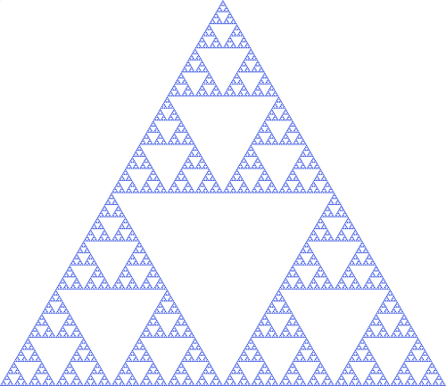
from https://commons.wikimedia.org/wiki/File:Sierpinski_triangle.svg

We can see that there are 3 copies of the whole when we apply a scaling factor of 1/2, or in other words, we can rebuild the entire fractal by using 3 copies that are scaled at 1/2.. Thus, M=3, S=1/2, so our equation becomes . We can take the log of each side to solve for d:

. Then we can bring the exponent down using the power rule to get . Now we can isolate d: and then take advantage of that fact that a negative sign multiplying log 1/2 is the same as taking the positive log of 2, so and so d= 1.585. This number tells us that the dimensionality of the Sierpinski triangle is somewhere between a line (1-d) and an area (2-d), which means dimensionality can exist as a non-integer. Furthermore, because the fractal dimension of the Sierpinski triangle is slightly over 1.5 , we can conclude that the Sierpinski triangle is slightly more 2 dimensional than 1 dimensional.

The following proof shows that the Sierpinski triangle is somewhere between 1 and 2 dimensions because its length (1st dimension) is infinite but its area (2nd dimension) is 0, according to the following proof:

Let’s start with area:

At each iteration of the Sierpiński triangle construction, the center 1/4 of each remaining triangle is removed, so 3/4 of the area is retained at each step.
Let denote the area of the original equilateral triangle, and let denote the total area remaining after iterations.
The area after steps is therefore given by

Since , it follows that

Therefore, the Sierpiński triangle has area zero.

We can also show how the Sierpinski triangle has infinite perimeter: Our initial perimeter is for a single equilateral triangle, for which each side has length L:

After the first Sierpiński iteration, there are 3 smaller triangles, each with 3 sides of length since each of the new equilateral triangles’ sides are constructed from the midpoint of L.
So the total perimeter after the first iteration is: .

After the second iteration, there are small triangles (at each iteration, every triangle gets divided into 3 triangles) each with 3 sides of length .
So , . In general, after iterations, the number of small triangles is , and the side length of each is . Hence . or, equivalently: .

Starting from , we take the limit as : . Since , the exponential grows without bound, so . Therefore .

From our calculations of perimeter and area, it seems that the perimeter increases more quickly to infinity than the area decreases towards 0, which yields the intuition that perhaps the Sierpinski triangle is more area-like than line-like, since for each successive iteration in the fractal we have the following relationship:

In other words, the perimeter increases by 50% while the area decreases by 25% after each iteration, meaning that the perimeter becomes infinite “faster” than the area gets to 0 so the Sierpinski seems to be more area-like.

This seems to hint that there is a way to calculate the fractal dimension based on how quickly perimeter increases relative to how quickly area decreases, and that if perimeter increases faster than area, then the fractal dimension should be above 1.5, showing it is closer to a 2d area than a 1d line.

In order to calculate the fractal dimension based on the relative increases and decreases of perimeter and area, we must first address how perimeters and areas generally scale according to their mass M (self-similar copies) and scaling factor s.

We can derive how perimeters generally scale by first using the Sierpinski triangle as an example. We assume it is built from M_n+1 triangle copies, each of whose 3L lengths is scaled by factor s compared to the previous step’s M_n copies, so our perimeter scaling after each consecutive iteration is The final equation , shows us the ratio of perimeters for any self-similar fractal and we are only left with the two terms: the ratio of tells us the factor we multiplied M_n by to get M_n+1, each of whose side lengths are s times those of the M_n copies. For the Sierpinski triangle specifically, since each consecutive iteration generates three times the number of copies as the previous step, and s=1/2, since each new copy is 1/2 the side length of the previous iteration. Using concrete numbers as an example, if M_n=1 and s=1/2, then M_n+1=3 copies, each of whose side lengths has been shrunken by 1/2, so that the total perimeter must now be = 3/2 the length of the previous iteration! And, since , each shrunken by 1/2, for every consecutive iteration, the total perimeter must always be 3/2 times the length of the previous iteration.

Our 2-d area scaling for the Sierpinski triangle and more generally for any self-similar fractal begins by scaling each of the 2 lengths needed to calculate area by s in each of the M_n+1 copies, so we get: where is the area scaling for any self-similar fractal in 2d space. For the Sierpinski triangle, we have , where each of the M_n+1 area copies has been scaled by , so for every consecutive iteration, the total area must be. =3/4 times the area of the previous iteration.

We can actually now figure out what s and are in terms of our perimeter and area iterations. Let’s first look at how to solve for s:

. This means that in terms of perimeter and area, .

Now we must solve for in terms of our perimeter and area iterations. From our previous discussion, we already know that

and solving for gives . Substituting in

we get that which when simplified becomes .

We are now ready to get our fractal dimension in terms of perimeter and area alone. As we already know, fractal dimension is ,, and so . We can now substitute our terms and . into our fractal dimension equation to obtain

In order to make more intuitive sense of this equation, let’s let and . Our equation, in terms of x and y, then becomes . We can transform this equation to give greater intuition by pulling out an x + y factor in the numerator : , which then can become , and plugging our original values back for x and y gets us our final version .

This final equation tells us that if the log ratio of the perimeter iteration is larger than the log ratio of the area iteration, we get a fractal dimension above 1.5, and thus more 2-d like than 1-d like, just as we predicted earlier. Let’s first get a deeper understanding of the denominator. The log of the area ratio is always negative, since A_n+1 is always less than A_n, so that when we subtract the term in the denominator, , we are actually always getting a positive number.. So the intuition of our expression is clearer now: it tells us the share of the total multiplicative change (log-based changes are multiplicative growth) that belongs to the change of the perimeter. If is greater than .5, the perimeter increased faster than the area decreased (in a multiplicative, log sense) and thus the fractal dimension will be above 1.5 and more area-like than line like; if is less than .5, the area decreased faster than the perimeter increased (in multiplicative growth), and thus the fractal dimension will be below 1.5 and more line-like than area-like.

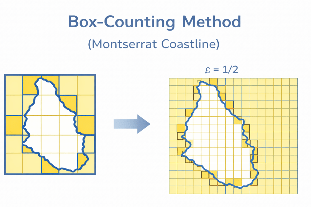
But what about when there is a fractal that does not contain self-similar copies? How can we measure the fractal dimension? After all, our fractal dimension formula depends on M, the number of self-similar copies. Thankfully, there is another ingenious way to measure fractal dimension: box counting. With box counting, we take an irregular form like a coastline and put it on a boxed grid, count the number of boxes that the coastline passes through, and then shrink our boxes to see how the image scales. Because there are no self similar copies contained within coastlines and other irregular patterns, the boxes themselves essentially become M, the number of copies, that we count.

The basic box counting formula (we will be modifying it shortly) is . N(ε) means the number of boxes of side length ε (which is always a fraction of the original box length of 1) that is intersected by the fractal shape. The symbol $\approx$ means “approximately equal to.” The exponent d is the box-counting fractal dimension. So the equation says that as the box size gets smaller, the number of boxes intersected by the fractal shape grows at a constant rate d, which is the fractal dimension. Note that this formula has the same structure as our mass scaling formula for self-similar fractals.

Let’s solve for d in our box counting formula:

Since $-\log(\varepsilon)=\log(1/\varepsilon)$, you can also write it as

Using the example of the Sierpinski triangle, we already know that when we use the mass-scaling formula for self similar fractals, we have 3 copies of the original, each copy shrunken by 1/2 length compared to the whole. Will the box counting method result in the same fractal dimension? Let’s use the more straightforward example of the Sierpinski Right triangle, formed using the same repetitive process of connecting midpoints and removing the middle 1/4 of each triangle. The Sierpinski right triangle makes the box counting method most clear. We assume we started with a box of side length 1 that had the entire triangle inside it, and then scaled that box with the scaling factors shown below:

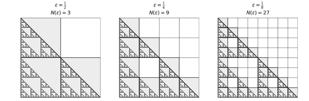
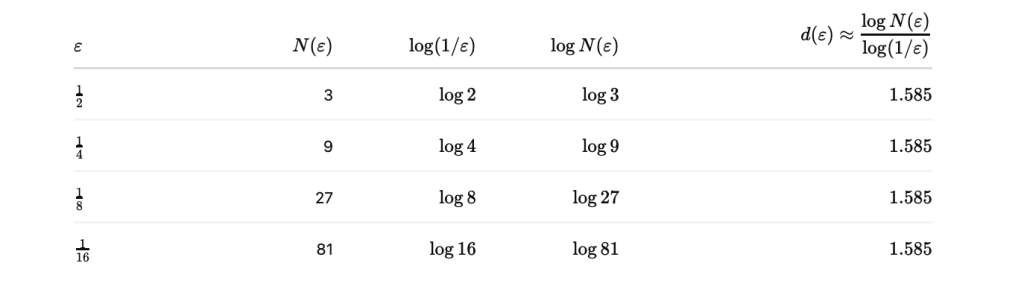
Here we see that we get exactly the same fractal dimension using the box counting method as we did using the fractal self-similar mass method, since each box maps perfectly to count exactly 1 self-similar copy of the fractal at every scale ! However, when we use the equilateral Sierpinski triangle, there is a slight difference in the fractal dimension calculation: as we shrink the box size , we get closer and closer to d=1.585, as shown below, rather than calculating d=1.585 at every scale:

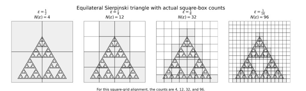
The above shows that our approximation to the true fractal dimension improves as so we must modify our box counting formula by including this limit: . As we are shrinking the boxes, we get a more and more accurate estimate because the number of infintesimally sized boxes match very closely with the infinitesimally sized fractal copies. In the case where a fractal lacks self-similar copies, such as an irregular coastline, the boxes themselves can be considered the number of copies, or mass, as the boxes continue to shrink.

There is one last modification we need to make to the box counting formula. The meaning of is that we have boxes of side length 1, and these are the original boxes to which we apply the different scaling factors of . If, for example, we started our box counting with 10 boxes of side length one, our box counting formula would be: , since when , we must get the correct number of boxes to equal 10, and then apply different scaling factors to those 10 boxes (resulting in 10 times the box count compared to starting with 1 box).

So our general box counting formula becomes , with c equal to the number of original boxes of side length one) and taking the log of both sides we get which becomes after applying some previously discussed log rules and rearranging.

Now solving for d we get and taking the limit as we get ,

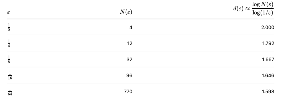
Let’s put this box counting formula to work by using the classic example of how to calculate the fractal dimension of the coastline of Great Britain:

We see from the above that the fractal dimension, or the slope of this line, is approximately 1.18, We know that the fractal dimension is the slope because the formula is with d representing the slope m in y = mx +b for a line. If we were to shrink for the coastline, we would not really be able to count boxes and we would be estimating things such as atoms and molecules, so practically we cannot actually take in using the box counting method for coastlines. Another problem we face in using box counting for coastlines is that depending on the range of scales, we may get different approximations for d, unlike for the Sierpinski Triangle. However, it is often cited that the fractal dimension of the coastline of Great Britain is around d1.25 since it maintains a remarkable consistency around a specific range of smaller scales where the log-log relationship remains approximately linear.

As promised, we finally return to the notion that this simple number, the fractal dimension of a coastline, can tell us so much about an island’s geological history. Below are some of the fractal dimensions calculated through the box counting method, where a specific range of smaller scales of the boxes reveals a relatively stable calculation for the fractal dimension:

Fractal Dimensions of Caribbean Coastlines

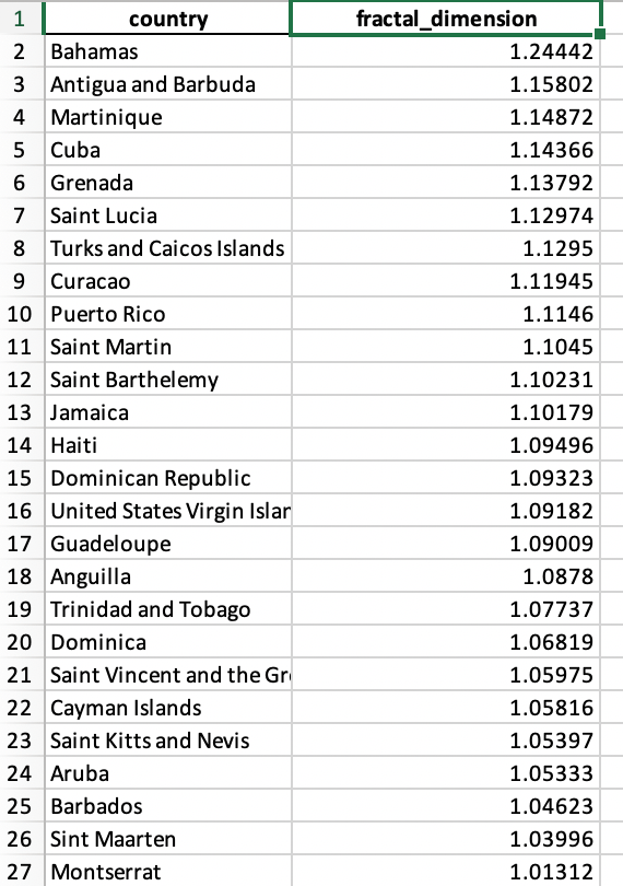
from https://datarepository.wolframcloud.com/resources/WolframSummerCamp_Coastline-Fractal-Dimensions/

We will use three of these groups of islands, the Bahamas (the highest fractal dimension on this list at d 1.24), the United States Virgin Islands ( a middling fractal dimension of d 1.09) and Montserrat (the lowest fractal dimension 1.01) to understand why the fractal dimensions of these coastlines carry an entire story with them.

The Bahamas has the highest fractal dimension of all the Caribbean islands at approximately 1.244, which makes sense for a low-lying archipelago built on shallow carbonate banks rather than a single steep island. The Bahamas is largely composed of limestone and carbonate, formed from the remains of coral and other marine skeletons. Much of the country sits on very shallow platforms, often 10 meters deep or less. That setting gives wave action more ways to create complexity: instead of hitting one direct shoreline, waves refract and break across the easy-to-erode, low lying carbonate banks, creating complex patterns due to the repeated iterations of wave action carving into the shoreline. It is this easily repeatable carving out of the Bahamas shoreline that makes its fractal dimension the highest out of all the islands.

The U.S. Virgin Islands sits in the middle of the list with a fractal dimension of approximately 1.092. The islands are mostly volcanic in origin, and were formed 100 million years ago. Because these islands were built by ancient volcanoes (which have not been active since), they contain steeper slopes along the coastlines than the Bahamas. Additionally, the volcanic rock is harder to erode than the carbonate of the Bahamas. These factors, namely the steeper slope and the harder-to-erode rock, make it harder for waves to carve out the shoreline. This helps explain why St. Thomas has a lower fractal dimension than the Bahamas.

Montserrat has the lowest fractal dimension value of approximately 1.013, suggesting a coastline that is comparatively smooth at the scale measured. This makes a lot of sense: similar to St. Thomas, Montserrat is built from volcanic action, but unlike St. Thomas, Montserrat has had very recent eruptions in which the coastline has been smoothed over by lava flows. Thus, in Montserrat, the very recent volcanic action has smoothed over many of the coastline irregularities, resulting in a very low fractal dimension closest to 1.

We can understand through these three examples that nature often forms fractals because of repetitive processes that iterate similar to the process that creates the Sierpinski triangle. In the case of the coastlines, we see that the repetitive process of waves crashing into the shoreline can create very intricate patterns, whose complexity increases depending on how amenable the geological structure is for waves to carve out patterns. The very complexity of this action means that we do not get self similar fractals that are produced with ideal mathematical constructions (like the Sierpinski Triangle), but rather we get imperfect and jagged structures whose dimensions are between 1 and 2. Nevertheless, we see that from our previous discussion, we can still calculate the fractal dimension of these imperfect shapes using the box counting method, which can produce a reliable estimate of how a coastline consistently behaves over defined ranges of scaling factors. Moreover, we now know that behind the box-counting of the coastlines lurks an even deeper principle: a race between the perimeter and area of the fractal, with perimeter ballooning to infinity and area shrinking to 0. It is this mathematical race that lies at the very foundation of understanding whether a fractal behaves more like a line or more like an area, and such understanding can extend to the inter-dimensionality of other fractal shapes as well. For instance, if we have a fractal shape between the second and third dimension , we can view such a shape’s fractal dimension as a race between its area ballooning to infinity and its volume shrinking to zero. Fractal dimension, then, is not just a number. It’s a way of describing where a shape lives within a dimensional race, and it’s nature’s way of revealing hidden structure.