Rolling the Dice: A Derivation of Schrodinger’s Equation from the Wave Equation

Waves and Young’s Double Slit Experiment

The quantum world reveals an astonishing truth: light, electrons, and indeed all matter in the universe — including ourselves — are described by mathematical wavefunctions that represent the probabilities of finding each particle in a particular location. These wavefunctions remain spread out until a measurement or interaction with the environment, which causes them to entangle with the environment, destroying observable interference and yielding a discrete location for the particle. Before exploring how matter exhibits wave-like behavior, we must first understand how Young, in 1804, seemed to prove that light itself was a wave, rather than a particle. His famous double slit experiment is shown below:

Young’s Double Slit Experiment, with Interference Pattern, from https://en.wikipedia.org/wiki/Double-slit_experiment#/media/File:Doubleslit.svg

When shining a light through a partition with two openings, Young observed that the projection on the back screen formed the characteristic interference patterns of waves, where we see light and dark bands signifying two separate waves either interfering constructively with each other (crests adding to crests or troughs adding to troughs) creating light bands, or destructively with each other (crests adding to troughs), creating dark bands. This type of pattern is a fundamental characteristic of the wave equation, which shows how waves can add linearly to each other (for more on the linearity of waves, see https://mathintuitions.com/2025/04/28/of-unwavering-importance-the-wave-equation-derivation/?preview_id=1449&preview_nonce=1c838f4945&preview=true&_thumbnail_id=1491). Later on in the 19th century, James Clerk Maxwell showed mathematically that light is indeed a wave: an electromagnetic wave (for Maxwell’s derivation, see https://mathintuitions.com/2025/06/25/how-the-curl-of-curl-gives-light-on-electromagnetic-waves-and-other-phenomena/?preview_id=1788&preview_nonce=6b97f120bc&preview=true&_thumbnail_id=1892 . But this was not the end of the story.

As Planck, Einstein, and other early twentieth-century physicists demonstrated, light and electrons are BOTH waves and particles! The picture below shows what happens when you shoot single electrons through double slits. Each individual electron or photon makes one discrete mark on the screen, showing its particle nature rather than wave nature. However, after firing many individual particles, the classic interference pattern emerges. What does this tell us? That until the particle is detected, it is acting as a probability wavefunction, passing through both slits simultaneously, interferes with itself after passing the slits, and finally shows up as a single dot in one of the characteristic bright bands. A single particle NEVER appears in the dark bands; the dark bands show those areas where the wavefunction interfered with itself as a wave, before it appeared as a discrete particle on the detector screen. Thus, as a wave function, the electron seems to be exploring all possible paths (it is not in any one definite location), until detection forces it to become localized; before detection, we can only speak about the probability amplitude describing where the electron might be found if measured. The wavefunction itself is this amplitude, whose squared, normalized magnitude gives the actual probability distribution of finding the particle at a certain location upon detection.

The Double-Slit Experiment with individual electrons fired, from https://commons.wikimedia.org/wiki/File:Double-slit.svg

The equation first developed to deal with the dual wave and particle nature demonstrated by the above experiment is Schrodinger’s Equation, which can be derived through the wave equation itself. As a reminder, the wave equation, in this case for an electromagnetic wave traveling at speed = c, is $\displaystyle \frac{\partial^{2}E}{\partial x^{2}} - \frac{1}{c^{2}}\frac{\partial^{2}E}{\partial t^{2}} = 0$ . A possible solution to this equation is a phase wave, $\displaystyle E(x,t) = E_0 e^{i(kx - \omega t)}$ , where E(x,t) is the amplitude of the wave at position x and time t, and $\displaystyle k\lambda = 2\pi \quad \text{and} \quad \lambda = \frac{2\pi}{k}$ . This shows that k influences wavelength: the higher k is, the smaller the wavelength (and vice-versa). Additionally, as the wave moves through time, we see that time is multiplied by a negative $\displaystyle \omega = 2\pi f$ , which means the wave moves to the right at w radians per second. An intuitive way to understand why -wt signifies a movement rightwards through time is that if we have a wave and we are at position $\pi$ and the wave is moving at 2 $\pi$ radians per second rightwards, that means that in one second, whatever the wave amplitude was at the position $-\pi$ has moved rightwards to our position $\pi$ (it has traveled 2 $\pi$ radians from $-\pi$ to $\pi$ ). This means that when we plug in our position, $\pi$ , we should get the amplitude that was -2 $\pi$ away from it: x-w(1s). Now if the wave traveled for t seconds, then our new phase would be at x-wt.

We can show that $\displaystyle E(x,t) = E_0 e^{i(kx - \omega t)}$ is a solution to the wave equation by takng its second derivative with respect to time and space, and then plugging those values back into the wave equation. With respect to time, the second derivative is $\displaystyle \frac{\partial^2 E}{\partial t^2} = \frac{\partial^2}{\partial t^2} \left( E_0 e^{i(kx - \omega t)} \right) = -\omega^2 E_0 e^{i(kx - \omega t)} = -\omega^2 E(x,t)$ and with respect to space, the second derivative is $\displaystyle \frac{\partial^2 E}{\partial x^2} = \frac{\partial^2}{\partial x^2} \left( E_0 e^{i(kx - \omega t)} \right) = -k^2 E_0 e^{i(kx - \omega t)} = -k^2 E(x,t)$ .

Plugging these values into the wave equation, we get the following:

$\displaystyle \frac{\partial^2 E}{\partial x^2} - \frac{1}{c^2}\frac{\partial^2 E}{\partial t^2} = 0 \;\Rightarrow\; (-k^2E) - \frac{1}{c^2}(-\omega^2E) = 0 \;\Rightarrow\; E\left(\frac{\omega^2}{c^2} - k^2\right) = 0 \;\Rightarrow\; \omega = ck$

This means that as long as w=ck, we have satisfied the wave equation! Let’s try to make sense of why it must be true that w=ck, in a more mathematically intuitive way. Firstly, we know that frequency times wavelength equals speed; for example, if a wave that is 10 meters long travels 5 wavelengths per second, that means it travels

10m/ $\displaystyle \lambda$ x 5 $\displaystyle \lambda$ /s = 50 meters per second! Now we know that the values of k and w (we will show w divided by c on each side) are the following: $\displaystyle k = \frac{2\pi}{\lambda}, \quad \frac{\omega}{c} = \frac{2\pi f}{c}$

Furthermore, we know that k=w/c, so we can then substitute: $\displaystyle \frac{2\pi}{\lambda} = \frac{2\pi f}{c}$ and solve for c: $\displaystyle c = \lambda f$ , which says that the speed equals frequency times wavelength, which matches what we would expect intuitively.

2. From Classical Waves to Quantum Energy and Momentum

Now that we have established a solution to the wave equation, we must adjust it according to the early 20th century developments in quantum mechanics in order to better understand the dual wave-particle nature of light. We can start our story with Max Planck, an early 20th-century physicist, who found that E=nhf, which states that the energy of radiation is equal to its frequency multiplied by Planck’s constant and n, where n is an integer. He introduced this idea to explain the behavior of the spectrum of blackbody radiation, though he still thought of light itself as a continuous wave. Planck’s formula for radiation, E=nhf, meant that the radiation was NOT absorbed or emitted continuously, but rather in discrete “quanta” — packets of energy proportional to the frequency of radiation. Classical physics, on the other hand, assumed that frequency did not matter for energy; rather, wave energy was seen to be dependent on intensity (which is reflected by light’s brightness and is defined by amplitude, or wave height). Then, Einstein proposed that light itself was composed of Planck’s discrete energy when he explained the cause of photoelectric effect: by increasing the frequency of light, you can eject more electrons from a metal surface, but you cannot eject more electrons by increasing its intensity (or wave amplitude). So whereas classical physics said that wave amplitude was the determinant for light’s energy, now, thanks to Planck and Einstein, we know that frequency is the determinant for light’s energy. Moreover, Einstein realized that when he applied Planck’s formula , the implication was that light is localized (acting like a particle) rather than spread out (acting like a wave). According to classical physics, the energy of light is spread out continuously across the wavefront, so an electron would need to absorb small amounts of this energy over time in order to be ejected. It might therefore take a measurable interval for the energy to build up sufficiently to eject the electron, but this never happens! Instead, because the electron was ejected instantaneously when light had a high enough frequency, Einstein realized that the energy transfer happens in quantized, instantaneous chunks — something only possible if light sometimes behaves as a particle of energy, which when packed with enough punch (a high enough frequency) can instantaneously eject the electron. Each individual particle’s energy is governed by Planck’s formula, E=nhf; n signifies a discrete number of photons, as opposed to a dispersed wave.

Not only did the definition of energy change, but so did the definition of momentum. In 1924, French physicist Louis de Broglie took Einstein’s idea of photons one step further. If light waves could behave like particles, he reasoned, perhaps particles of matter could also behave like waves. He proposed that every moving particle has an associated wavelength given by $\lambda = \frac{h}{p}$ where h is Planck’s constant and p is the particle’s momentum. He derived this equation by first using Einstein’s theory of special relativity and its definition of momentum:

2.5. Derivation of Particle Momentum using Relativity

$\text{The four-velocity is } u^\mu = \frac{dx^\mu}{dT}, \text{ and the four-momentum is } p^\mu = m u^\mu.$ , since to obtain momentum we must multiply velocity by mass m.

$dT \text{ (or } d\tau \text{) is the proper time measured in the particle's own rest frame.}$ So the full expression for momentum becomes:

$\displaystyle p^\mu = m\left(\frac{dx^0}{dT},\,\frac{dx^1}{dT},\,\frac{dx^2}{dT},\,\frac{dx^3}{dT}\right)$

where $\text{where } x^0 = ct,\; x^1 = x,\; x^2 = y,\; x^3 = z.$

For an observer outside the particle’s rest frame, we know that the ratio of his time dt to the proper time dT is $\displaystyle \frac{dt}{dT} = \frac{1}{\sqrt{1 - \frac{v^2}{c^2}}}$ , and solving for dT, we obtain:

$\displaystyle dT = dt\,\sqrt{1 - \frac{v^2}{c^2}}$ (for the Lorentz factor derivation, see https://mathintuitions.com/2025/01/23/the-lorentz-factor-and-the-invariance-of-relativity/?preview_id=1344&preview_nonce=31a655297f&preview=true&_thumbnail_id=1758)

We can now substitute the above expression for dT in $\displaystyle p^\mu = m\left(\frac{dx^0}{dT},\,\frac{dx^1}{dT},\,\frac{dx^2}{dT},\,\frac{dx^3}{dT}\right)$ to obtain:

$\displaystyle p^\mu = m\left(\frac{dx^0}{dt\sqrt{1-\frac{v^2}{c^2}}},\,\frac{dx^1}{dt\sqrt{1-\frac{v^2}{c^2}}},\,\frac{dx^2}{dt\sqrt{1-\frac{v^2}{c^2}}},\,\frac{dx^3}{dt\sqrt{1-\frac{v^2}{c^2}}}\right)$ , and when substituting for the Lorentz factor we get

$\displaystyle p^\mu=\gamma m\left(\frac{dx^0}{dt},\,\frac{dx^1}{dt},\,\frac{dx^2}{dt},\,\frac{dx^3}{dt}\right),\ \ \gamma=\frac{1}{\sqrt{1-\frac{v^2}{c^2}}}$ ,

Furthermore, knowing that $\displaystyle (x^0,x^1,x^2,x^3)=(ct,\,x,\,y,\,z)\ \text{and}\ (v_x,v_y,v_z)=\left(\frac{dx}{dt},\,\frac{dy}{dt},\,\frac{dz}{dt}\right)$

we can express momentum as

$\displaystyle p^\mu=\gamma m\left(\frac{dx^0}{dt},\,\frac{dx^1}{dt},\,\frac{dx^2}{dt},\,\frac{dx^3}{dt}\right)=\gamma m\left(\frac{d(ct)}{dt},\,\frac{dx}{dt},\,\frac{dy}{dt},\,\frac{dz}{dt}\right)=\gamma m(c,\,v_x,\,v_y,\,v_z),\ \ \gamma=\frac{1}{\sqrt{1-\frac{v^2}{c^2}}}$

The above expression gives momentum as a 4 vector, and is now in terms of the observer’s time dt- much more intuitive compared to the proper time dT, which is more difficult to grasp intuitively since it would only belong to the clock traveling with the moving particle. We see from the equation that that the zeroth component for momentum actually equals E/c, because of the following relation:

$\displaystyle P^0 = \gamma m c = \frac{E}{c}, \quad \text{where } E = \gamma m c^2$

DeBroglie then used E=hf to make some substitutions for momentum, shown below, for photons and other massless particles:

$\displaystyle P^0=\frac{E}{c}=\frac{h f}{c}=\frac{h}{\lambda}$

Although at first glance it appears that only the zeroth component of momentum equals $h/\lambda$ only for massless particles, Lorentz invariance requires energy–momentum and frequency–wavevector to transform consistently as four-vectors (see the appendix entitled Understanding the Invariance of the Klein-Gordon Equation). While neither momentum nor wavelength is itself invariant, this relation holds for all matter in all inertial frames, and may be written in any given frame as $p=h/\lambda$ where $\lambda$ is the de Broglie wavelength (for more on Lorentz invariance see, https://mathintuitions.com/2025/01/23/the-lorentz-factor-and-the-invariance-of-relativity/?preview_id=1344&preview_nonce=a649a25931&preview=true&_thumbnail_id=1758).

3. From the Wave Equation to the Klein-Gordon Equation

In the light of Planck’s and Einstein’s discoveries, we can now modify our wave equation knowing that E=hf and $\displaystyle p = \frac{h}{\lambda}$ . Firstly, we would like to express everything in terms of radians to gain a better understanding of the wave phase, which tells us where the wave is in its cycle of time and space. To accomplish this, we can modify E=hf by substituting $\hbar = \frac{h}{2\pi}$ and $\omega = 2\pi f$ to obtain $E = \hbar \omega$ . This means that $\omega = \frac{E}{\hbar}$ . Similary, for our momentum expression $\displaystyle p = \frac{h}{\lambda}$ , we can substitute $k = \frac{2\pi}{\lambda}$ into our momentum equation to get $p = \hbar k$ , where again $\hbar = \frac{h}{2\pi}$ . This means that $k = \frac{p}{\hbar}$ . We can now substitute for w and k in our original equation, which is $\displaystyle \psi=\psi_{0}\,e^{i(kx-\omega t)}$ with $\displaystyle \psi_{0}$ as the amplitude of the wave. After substituting, this equation becomes $\displaystyle \psi=\psi_{0}\,e^{\tfrac{i}{\hbar}(px-Et)}$ , where $\psi(x,t)$ is the wavefunction in terms of variables x and t and no longer only needs to represent an electric field, but any wave.

Plugging this into our wave equation, we get $\displaystyle \psi=\psi_{0}e^{\tfrac{i}{\hbar}(px-Et)}\;\Rightarrow\;\frac{\partial^2\psi}{\partial x^2}-\frac{1}{c^2}\frac{\partial^2\psi}{\partial t^2}=\left(-\frac{p^2}{\hbar^2}+\frac{1}{c^2}\frac{E^2}{\hbar^2}\right)\psi=\frac{1}{\hbar^2}\left(\frac{E^2}{c^2}-p^2\right)\psi=0$ .

This confirms that $\displaystyle p=\frac{E}{c}.$ when there is no mass involved like photons. However, we must also consider cases in which there is mass.

In order to address this, we can first contract the contravariant components of P with its covariant components in order to get a scalar invariant (more on this idea to come in a future post, but for now familiarity with tensors is required to understand the next idea). To figure out the covariant components of momentum, we can multiply the contravariant components by the Minkowski metric tensor for flat space, which is +1, -1, -1, -1, and then contract our contravariant and covariant components:

$\displaystyle p^\mu = (\gamma m c,\gamma m v_x,\gamma m v_y,\gamma m v_z),\;p_\mu = (\gamma m c,-\gamma m v_x,-\gamma m v_y,-\gamma m v_z),\;\Rightarrow\;p_\mu p^\mu = (\gamma m c)^2-\gamma^2 m^2(v_x^2+v_y^2+v_z^2)=\gamma^2 m^2(c^2-v^2)=m^2 c^2,\;\text{where }\gamma=\frac{1}{\sqrt{1-\frac{v^2}{c^2}}}.$

So now we can make use of two results of the momentum contraction:

$\displaystyle p_{\mu}p^{\mu}=(\gamma mc)^{2}-\gamma^{2}m^{2}(v_{x}^{2}+v_{y}^{2}+v_{z}^{2})=\frac{E^{2}}{c^{2}}-p^{2},\;\;E=\gamma mc^{2}$ and

$\displaystyle p_{\mu}p^{\mu}=m^{2}c^{2}$

and set them equal to each other to solve for the energy term:: we get $\displaystyle p_\mu p^\mu=\frac{E^2}{c^2}-p^2=m^2c^2\;\Rightarrow\;E^2=p^2c^2+m^2c^4\;\Rightarrow\;E=\sqrt{p^2c^2+m^2c^4}\,.$ ; when we have a photon, m=0 and the second term vanishes, and we plug in E=hf for energy and $\displaystyle p=\frac{h}{\lambda}$ for momentum, but when we have an object with mass we also include the second term.

We can now plug this into our wave equation, which for massless particles is :

$\displaystyle -\frac{1}{\hbar^{2}}\left(p^{2}-\frac{E^{2}}{c^{2}}\right)\psi = 0.$ , but for objects with mass, we must include the full energy term:

$\displaystyle E^{2}=p^{2}c^{2}+m^{2}c^{4}\;\Rightarrow\;\frac{E^{2}}{c^{2}}=p^{2}+m^{2}c^{2}\;\Rightarrow\;p^{2}-\frac{E^{2}}{c^{2}}+m^{2}c^{2}=0$ and plugging that in for the values inside the parentheses that must equal 0, we get $\displaystyle -\frac{1}{\hbar^{2}}\left(p^{2}-\frac{E^{2}}{c^{2}}+m^{2}c^{2}\right)\psi = 0.$ .

We can further rewrite the momentum and energy terms in the above equation by treating them not as independent parameters, but as operators acting on the wavefunction, reflecting the fact that momentum and energy are encoded in the wave’s spatial and temporal oscillations. In the above equation, we see that energy and momentum are one discrete quantity, but most wavefunctions contain many independent waves, each with their own energy and momentum, so the energy and momentum operators can extract these across many linear combinations of waves. Starting with our wavefunction, $\displaystyle \psi(x,t)=\psi_{0}\,e^{\tfrac{i}{\hbar}(px-Et)}$ , where $\displaystyle \psi_{0}$ is our amplitude of the wave, we get

$\displaystyle \frac{\partial}{\partial x}\left(\psi_{0}e^{\tfrac{i}{\hbar}(px-Et)}\right)=\frac{i\,p}{\hbar}\,\psi_{0}e^{\tfrac{i}{\hbar}(px-Et)}$

and after multiplying each side by $\displaystyle -i\hbar$ we get:

$\displaystyle p\,\psi_{0}e^{\tfrac{i}{\hbar}(px-Et)}=-\,i\hbar\,\frac{\partial}{\partial x}\left(\psi_{0}e^{\tfrac{i}{\hbar}(px-Et)}\right)$ . Finally, we can substitute in our wave function, $\displaystyle \psi(x,t)=\psi_{0}\,e^{\tfrac{i}{\hbar}(px-Et)}$ , where $\displaystyle \psi_{0}$ , to get:

$\displaystyle p\,\psi=-i\hbar\,\frac{\partial\psi}{\partial x}$ .

If we repeat the previous sequence by taking the derivative with respect to x and then multiplying each side by ih, we get:

$\displaystyle p^{2}\psi=-\hbar^{2}\,\frac{\partial^{2}\psi}{\partial x^{2}}$

Now let’s do the same for energy:

$\displaystyle \frac{\partial}{\partial t}\left(\psi_{0}e^{\tfrac{i}{\hbar}(px-Et)}\right)=-\,\frac{i\,E}{\hbar}\,\psi_{0}e^{\tfrac{i}{\hbar}(px-Et)}$ , so

$\displaystyle E\,\psi_{0}e^{\tfrac{i}{\hbar}(px-Et)}=i\hbar\,\frac{\partial}{\partial t}\left(\psi_{0}e^{\tfrac{i}{\hbar}(px-Et)}\right)$ and after substituting in our wave function $\displaystyle \psi(x,t)=\psi_{0}\,e^{\tfrac{i}{\hbar}(px-Et)}$ , we get:

$\displaystyle E\,\psi=i\hbar\,\frac{\partial\psi}{\partial t}$

If we repeat the previous sequence by taking the derivative with respect to t and then once again multiplying each side by ih, we get:

$\displaystyle E^{2}\psi=-\hbar^{2}\,\frac{\partial^{2}\psi}{\partial t^{2}}$

In terms of operators on the phase wave and considering more than 1 dimenison, we get

$\displaystyle \hat{p}=-\,i\hbar\,\nabla$ and $\displaystyle \hat{E}=i\hbar\,\frac{\partial}{\partial t}$ , where the spatial and time derivatives are assumed to be acting on the wavefunction. These operators, when applied twice to the wave function, are squared (note that the derivative operator squared signifies taking the derivative twice, or in other words taking the second derivative), can extract the individual energy squared and momentum squared terms from each of the individual plane waves, which are linear contributions to the overall wavefunction.

Plugging in these for our energy and momentum in $\displaystyle -\frac{1}{\hbar^{2}}\left(p^{2}-\frac{E^{2}}{c^{2}}+m^{2}c^{2}\right)\psi = 0.$ , we get

$\displaystyle -\frac{1}{\hbar^{2}}\left[(-i\hbar\nabla)^{2}-\frac{(i\hbar\,\partial/\partial t)^{2}}{c^{2}}+m^{2}c^{2}\right]\psi=0$ .

Redistributing and cancelling yields:

$\displaystyle \left(\nabla^{2}-\frac{1}{c^{2}}\frac{\partial^{2}}{\partial t^{2}}-\frac{m^{2}c^{2}}{\hbar^{2}}\right)\psi=0$

This equation is called the Klein-Gordon equation, which is the relativistically invariant wave equation that combines quantum mechanics with special relativity. Please see the appendix called Understanding the Invariance of the Klein-Gordon Equation to understand more about how the phase wave is invariant, and energy and momentum are relativistically invariant.

From the Klein-Gordon equation, we will now attempt to derive the Schrodinger Equation, which is non-relativistic and relies on low speeds. We start by modifying our energy term $\displaystyle E = \sqrt{p^2c^2 + m^2c^4}$ . Then we can factor out an $\displaystyle mc^2$ to obtain $\displaystyle E = mc^2\sqrt{1 + \frac{p^2}{m^2c^2}}$ . The next step is to Taylor expand $\displaystyle \sqrt{1 + \frac{p^2}{m^2c^2}}$ around x=0, where the term x= $\displaystyle \frac{p^2}{m^2c^2}$ is very small, since the velocity in p=mv is dwarfed by the speed of light, c, in the denominator; expanding all the derivatives around x=0 and then taking a tiny step to x= $\displaystyle \frac{p^2}{m^2c^2}$ should give us a very good approximation.

$\displaystyle f(x)=\sqrt{1+x},\; f'(x)=\tfrac12(1+x)^{-1/2},\; f''(x)=-\tfrac14(1+x)^{-3/2},\; f'''(x)=\tfrac38(1+x)^{-5/2}$

Now evaluating at x=0 yields:

$\displaystyle f(0)=1,\; f'(0)=\tfrac12,\; f''(0)=-\tfrac14,\; f'''(0)=\tfrac38$

We can plug these values for the function and derivatives into the general Taylor series, which is

$\displaystyle f(x)\approx f(0)+f'(0)\,x+\frac{f''(0)}{2!}x^2+\frac{f'''(0)}{3!}x^3$ , and instead of x, we assume very small variations in the variable $\displaystyle \frac{p^2}{m^2c^2}$ where energy is a function of p and the aforementioned $\displaystyle \frac{p^2}{m^2c^2}$ term has been Taylor expanded around p=0:

$\displaystyle E(p)=mc^2\sqrt{1+\frac{p^2}{m^2c^2}}$

$\displaystyle E(p)\approx mc^2\Big[1+\frac{1}{2}x-\frac{1}{8}x^2+\frac{1}{16}x^3\Big]=mc^2\Big[1+\frac{1}{2}\frac{p^2}{m^2c^2}-\frac{1}{8}\Big(\frac{p^2}{m^2c^2}\Big)^2+\frac{1}{16}\Big(\frac{p^2}{m^2c^2}\Big)^3\Big]\approx mc^2+\frac{p^2}{2m}-\frac{p^4}{8m^3c^2}+\frac{p^6}{16m^5c^4},\quad x=\frac{p^2}{m^2c^2}$ .

We are only really interested in the first two terms above in the approximation, since the higher order terms quickly go to 0 with the assumption of a very small $\displaystyle \frac{p^2}{m^2c^2}$ .

The second term of the above series is actually the kinetic energy, since $\displaystyle \frac{p^2}{2m} = \frac{1}{2}mv^2$ , being that p=mv in nonrelativistic physics, so our energy term becomes the first two terms of our Taylor series, $\displaystyle E = mc^2 + \text{K}$ , where K represents the classical kinetic energy.

We can now return to our Klein Gordon equation and begin to rewrite it with this new knowledge. The Klein-Gordon equation is $\displaystyle \nabla^{2}\Psi - \frac{1}{c^{2}}\frac{\partial^{2}\Psi}{\partial t^{2}} - \frac{m^{2}c^{2}}{\hbar^{2}}\,\Psi = 0$ , where $\displaystyle \Psi(x,t)=\Psi_{0}e^{\frac{i}{\hbar}(px-Et)}$ , and $\displaystyle \psi_0$ is a constant to modify the amplitude of the wave.

Plugging $\displaystyle E = mc^2 + \text{K}$ into our energy term in $\displaystyle \Psi(x,t)=\Psi_{0}e^{\frac{i}{\hbar}(px-Et)}$ , we get $\displaystyle \Psi(x,t)=\Psi_{0}e^{\frac{i}{\hbar}(px-mc^2 t-Kt)}=e^{-\frac{i}{\hbar}mc^2 t}\,\Psi_{0}e^{\frac{i}{\hbar}(px-Kt)}$ . Now to understand why we pulled the term
$\displaystyle e^{-\frac{i}{\hbar}mc^2 t}$ out as its own factor requires a “quantum leap” in conceptual understanding, thanks to the physicist Max Born.

4. Born’s Interpretation and Normalization of the Wave Function

Max Born reinterpreted the wavefunction $\displaystyle \Psi(x,t)$ not as a physical wave spread out in space, but as a probability amplitude. He was led to this view by experiments such as electron diffraction and the double-slit experiment, which revealed the profound puzzle we already discussed: that quantum particles exhibit wave-like interference patterns, yet they are always detected as localized particles. The wavefunction itself could not represent a physical, smeared-out electron since it is always detected at a single location, but its squared, normalized magnitude matched the observed statistical frequencies of detection events. Since the wavefunction is generally complex-valued, only the wavefunction multiplied by its complex conjugate $\displaystyle |\Psi(x,t)|^2 = \Psi^*(x,t)\Psi(x,t)$ yields a real, non-negative quantity that can be interpreted as a probability density. Next Born realized that we must set the integral of the probability density, shown by the squared value of the wave function, over all possible locations to 1, implying a 100 % chance that the quantum particle would have to appear somewhere in space. Remarkably, this interpretation not only resolved the wave–particle dilemma but also matched experimental results with extraordinary accuracy.

Therefore, the total probability of finding a particle somewhere in space is given by

$\displaystyle \int_{-\infty}^{\infty} \Psi^*(x,t)\Psi(x,t)dx = 1,$ where the integrand is the product of the wavefunction and its complex conjugate. If we compute this integral and obtain a value other than 1 — for example, $\displaystyle 5$ — then the wavefunction is not normalized. To fix this, we divide the wavefunction by $\displaystyle \sqrt{5}$ so that the new integral becomes 1, since the square root term would appear under both $\displaystyle \Psi(x,t)$ and $\displaystyle \Psi^*(x,t)$ and multiplying each of these factors would equal 5 in the denominator.

Now we can return to the equation $\displaystyle \Psi(x,t)=\Psi_{0}e^{\frac{i}{\hbar}(px-mc^2 t-Kt)}=e^{-\frac{i}{\hbar}mc^2 t}\,\Psi_{0}e^{\frac{i}{\hbar}(px-Kt)}$ to better understand why we rewrote it with the $\displaystyle e^{-\frac{i}{\hbar}mc^2 t}$ pulled out. We can firstly see that this factor multiplies the wave by the extremely high angular frequency of $\displaystyle \omega = \frac{mc^2}{\hbar}$ at every point in space at a given time; however, ultimately this factor does not affect the probability density at all!

Because our probability density is defined as $\displaystyle \int_{-\infty}^{\infty} \Psi^*(x,t)\Psi(x,t),dx = 1.$ we can see why the term $\displaystyle e^{-\frac{i}{\hbar}mc^2 t}$ has no effect at all based on the fact that we are multiplying the wavefunction and its complex conjugate (which is found by flipping the sign in front of the imaginary number, i), so that the sign of the imaginary exponent flips, and the two factors cancel:

$\displaystyle e^{+\frac{i}{\hbar}mc^2 t}e^{-\frac{i}{\hbar}mc^2 t} = 1$ .

Therefore, the rapidly oscillating term does not affect the probability density since it multiplies to 1 inside the integral that multiplies the wave function and its conjugate, which is designated with the bar over it:

$\displaystyle \int_{-\infty}^{\infty} \left(\overline{e^{+\frac{i}{\hbar}mc^2 t}\Psi(x,t)}\right)\left(e^{+\frac{i}{\hbar}mc^2 t}\Psi(x,t)\right)\,dx = \int_{-\infty}^{\infty} \left(e^{-\frac{i}{\hbar}mc^2 t}\,\overline{\Psi(x,t)}\right)\left(e^{+\frac{i}{\hbar}mc^2 t}\Psi(x,t)\right)\,dx = \int_{-\infty}^{\infty} \overline{\Psi(x,t)}\Psi(x,t)\,dx = 1.$ , remembering that the integrand has been normalized to one.

To more simply calculate derivatives, we can redefine our wave function as $\displaystyle \Psi = e^{-\frac{i mc^2 t}{\hbar}} \phi$ , where $\displaystyle \phi = \Psi_0 e^{\frac{i}{\hbar}(px - Kt)}$ . Since the global phase $e^{-i mc^2 t/\hbar}$ has no effect on the probability density as we previously established, we can equally well impose the normalization condition on ϕ so now the probability density condition can be expressed as:

$\displaystyle \int_{-\infty}^{\infty} \phi^*(x,t)\,\phi(x,t)\,dx = 1$

Our first derivative of $\displaystyle \Psi = e^{-\frac{i mc^2 t}{\hbar}} \phi$ , respect to time is:

$\displaystyle \frac{\partial \Psi}{\partial t} = -\frac{i mc^2}{\hbar} e^{-\frac{i mc^2 t}{\hbar}} \phi + e^{-\frac{i mc^2 t}{\hbar}} \frac{\partial \phi}{\partial t}$

and our second derivative with respect to time is therefore:

$\displaystyle \frac{\partial^2 \Psi}{\partial t^2} = (-\frac{m^2 c^4}{\hbar^2} e^{-\frac{i mc^2 t}{\hbar}} \phi - \frac{2 i mc^2}{\hbar} e^{-\frac{i mc^2 t}{\hbar}} \frac{\partial \phi}{\partial t}) + e^{-\frac{i mc^2 t}{\hbar}} \frac{\partial^2 \phi}{\partial t^2}$

We can prove that the final term above, $\displaystyle e^{-\frac{i mc^2 t}{\hbar}} \frac{\partial^2 \phi}{\partial t^2}$ , is so much smaller than the first derivate term, such that we can discount the final term completely from the equation. To understand why, lets calculate what those first and second derivatives would be given $\displaystyle \phi = \Psi_0 e^{\frac{i}{\hbar}(px - Kt)}$ :

$\displaystyle \frac{\partial \phi}{\partial t} = -\frac{iK}{\hbar}\,\phi$

and

$\displaystyle \frac{\partial^2 \phi}{\partial t^2} = -\frac{K^2}{\hbar^2}\,\phi$

Now, let’s take the absolute value (only the relative absolute size matters) of the ratio of the second derivative term to the first derivative term, along with their coefficients in the equation:

$\displaystyle \frac{\left|e^{-\frac{i mc^2 t}{\hbar}}\frac{\partial^2\phi}{\partial t^2}\right|}{\left|\frac{mc^2}{\hbar}e^{-\frac{i mc^2 t}{\hbar}}\frac{\partial\phi}{\partial t}\right|}=\frac{\left|\frac{K^2}{\hbar^2}\phi\right|}{\left|\frac{mc^2}{\hbar}\frac{K}{\hbar}\phi\right|}=\frac{K}{mc^2}\ll1$

where the kinetic energy is much smaller than the denominator since we are assuming much lower speeds (non relativistic assumption) compared to the speed of light.

Thus, leaving out the negligibly small final term, our equation becomes:

$\displaystyle \frac{\partial^2 \Psi}{\partial t^2} = e^{-\frac{i mc^2 t}{\hbar}} \left[ -\frac{m^2 c^4}{\hbar^2}\phi - \frac{2 i m c^2}{\hbar}\frac{\partial \phi}{\partial t} \right]$

We can now return to our Klein-Gordon equation, which is $\displaystyle \nabla^{2}\Psi - \frac{1}{c^{2}}\frac{\partial^{2}\Psi}{\partial t^{2}} - \frac{m^{2}c^{2}}{\hbar^{2}}\,\Psi = 0$ and begin to plug in our values.

Our value for the 2nd derivative of the wave function with respect to space is :

$\displaystyle \nabla^2\Psi(x,y,z,t) = e^{-\frac{i mc^2 t}{\hbar}}\left(\frac{\partial^2 \phi}{\partial x^2} + \frac{\partial^2 \phi}{\partial y^2} + \frac{\partial^2 \phi}{\partial z^2}\right)$ and so we can plug this and our 2nd derivative with respect to time into the Klein Gordon equation:

$\displaystyle e^{-\frac{i mc^2 t}{\hbar}}\nabla^2\phi - \frac{1}{c^{2}}e^{-\frac{i mc^2 t}{\hbar}}\left[-\frac{m^2 c^4}{\hbar^2}\phi - \frac{2 i m c^2}{\hbar}\frac{\partial \phi}{\partial t}\right] - \frac{m^{2}c^{2}}{\hbar^{2}}e^{-\frac{i mc^2 t}{\hbar}}\phi = 0$

after dividing by $\displaystyle e^{-\frac{i mc^{2} t}{\hbar}} \, \nabla^{2}\phi$ and distributing $\displaystyle \frac{1}{c^{2}}$ , we get:

$\displaystyle \nabla^{2}\phi+\frac{m^{2}c^{2}}{\hbar^{2}}\phi-\frac{2im}{\hbar}\frac{\partial\phi}{\partial t}-\frac{m^{2}c^{2}}{\hbar^{2}}\phi=0$

We can further simplify by eliminating the terms that subtract to 0:

$\displaystyle \nabla^{2}\phi - \frac{2im}{\hbar}\frac{\partial\phi}{\partial t} = 0$

We can add a term on each side to get:

$\displaystyle \nabla^{2}\phi = \frac{2im}{\hbar}\frac{\partial\phi}{\partial t}$

and multpily by $\displaystyle i\hbar^{2}$ on each side after solving for $\displaystyle \frac{d\phi}{dt}$

$\displaystyle i\hbar\,\frac{\partial\phi}{\partial t} = -\frac{\hbar^{2}}{2m}\,\nabla^{2}\phi$ with the requirement that $\displaystyle \int_{-\infty}^{\infty} \phi^{*}(x,t)\,\phi(x,t)\,dx = 1$ .

This is the form of the Schrodinger equation we wanted because the left hand side actually expresses the kinetic energy. It shows energy because, firstly, as we know from Planck, $\displaystyle E = \hbar \omega$ . Our phase wave is defined as $\displaystyle \phi = \Psi_0 e^{\frac{i}{\hbar}(px - Kt)}$ . and its derivative with respect to time is

$\displaystyle \frac{\partial \phi}{\partial t}= -\frac{iK}{\hbar}\,\Psi_0 e^{\frac{i}{\hbar}(px - Kt)}$

$\displaystyle \frac{\partial \phi}{\partial t}= -\frac{iK}{\hbar}\,\phi$

After multiplying by $\displaystyle i\hbar$ , we get

$\displaystyle i\hbar \frac{\partial \phi}{\partial t}= K\,\phi$ , which shows that the left hand side of our Schrodinger equation, $\displaystyle i\hbar\,\frac{\partial\phi}{\partial t} = -\frac{\hbar^{2}}{2m}\,\nabla^{2}\phi$ , is exactly equal to the kinetic energy times the wave (we are assuming here that there is zero potential energy).

Schrödinger’s equation builds probability directly into time evolution, and is useful for measurements made in nonrelativistic, slow-speed quantum mechanics . The Klein–Gordon equation, by contrast, describes relativistic fields rather than particles, and probability only enters after the theory is quantized and measurements are defined.

Schrodinger’s equation is a fascinating equation that demonstrates the inherently probabilistic nature of the wave function, and possibly nature itself.

This post was inspired by https://chem542.class.uic.edu/wp-content/uploads/sites/720/2020/08/SEDerivation.pdf , which shows a derivation of the Schrodinger equation from the Klein-Gordon equation

APPENDIX: Understanding the Invariance of the Klein-Gordon Equation

The energy and momentum terms given by the Klein-Gordon equation as spatial and temporal derivatives are relativistically invariant, (measurements of space and time do depend on velocity of observer) but the wave phase is truly invariant no matter what inertial frame the observer is in.

We can show how the wave phase px-Et is invariant by first showing the relations between the invariant speed of light and the wave phase first expressed as kx – wt. Every frame must calculate that the speed of a wave equals frequency times wavelength, or in terms of k, w, and c (if our wave is traveling at the invariant speed of light c), then the relationship must be $\displaystyle c=\frac{\omega}{k}$ , even if w and k can vary (we will assume that w and k, like x and t, can be different for different frames). From the phase wave, we see that the phase is written in terms of kx-wt; we can now prove why kx-wt must be invariant, no matter the inertial frame, based on the fact that $\displaystyle \frac{\omega}{k}=c \;=\; \frac{\omega'}{k'}$ .

To first understand the invariance of kx-wt, let’s assume that our space and time coordinates can transform (as we know they do from https://mathintuitions.com/2025/01/23/the-lorentz-factor-and-the-invariance-of-relativity/. We will also assume for now that it’s possible for k and w to transform, so our new phase is k’x’ -w’t’. Now we must see why this phase must equal the kx-wt phase in a different frame. To do so, we will assume that k’x’-w’t’ can be expressed as kx-wt plus another angle function in terms of x and t: $\displaystyle e^{\,i(k'x' - \omega' t')} \;=\; e^{\,i(kx - \omega t + \theta(x,t))}$ .

First derivatives: $\displaystyle \frac{\partial}{\partial x}e^{\,i(kx-\omega t+\theta)}=i(k+\theta_x)e^{\,i(kx-\omega t+\theta)},\;\frac{\partial}{\partial t}e^{\,i(kx-\omega t+\theta)}=-i(\omega-\theta_t)e^{\,i(kx-\omega t+\theta)}$ . To find the second derivatives, we take advantage of the product rule with f(x) representing the factor with the i and g(x) representing the factor with base e:

$\displaystyle \frac{\partial^2}{\partial x^2}e^{\,i(kx-\omega t+\theta)}=\Big[i\,\frac{d^2\theta}{dx^2}-(k+\frac{d\theta}{dx})^2\Big]e^{\,i(kx-\omega t+\theta)},\;\frac{\partial^2}{\partial t^2}e^{\,i(kx-\omega t+\theta)}=\Big[i\,\frac{d^2\theta}{dt^2}-(\omega-\frac{d\theta}{dt})^2\Big]e^{\,i(kx-\omega t+\theta)}$

Plugging these derivatives into the wave equation, we get

$\displaystyle \Big[i\,\frac{d^2\theta}{dx^2}-(k+\frac{d\theta}{dx})^2\Big]e^{\,i(kx-\omega t+\theta)}-\frac{1}{c^2}\Big[i\,\frac{d^2\theta}{dt^2}-(\omega-\frac{d\theta}{dt})^2\Big]e^{\,i(kx-\omega t+\theta)}=0$

Gathering the real and imaginary terms, since only reals and imaginaries can be added to each other alone, we get:

$\displaystyle i\Big(\frac{d^2\theta}{dx^2}-\frac{1}{c^2}\frac{d^2\theta}{dt^2}\Big)-\Big[(k+\frac{d\theta}{dx})^2-\frac{1}{c^2}(\omega-\frac{d\theta}{dt})^2\Big]=0$

Solving for c, we get:

$\displaystyle c=\frac{\omega-\frac{d\theta}{dt}}{\,k+\frac{d\theta}{dx}\,}$ , which means that we do not recover the same speed of light as c=w/k , which disobeys physics. $\displaystyle \text{Only when } \frac{d\theta}{dx}=0 \text{ and } \frac{d\theta}{dt}=0 \text{ does it simplify to the usual invariant } c=\frac{\omega}{k}$ , which implies only with the addition of a constant theta (or a value of zero for theta) do we recover the invariant c . This means that every wave from every inertial frame must be in the same phase, unless shifted by a constant theta that is merely due to a difference in starting times or ascribing origins to different points. For example, if my origin is pi/2 ahead of yours, then I would subtract pi/2 from your position to shift the wave pi/2 to the right in my frame.

This means that kx-wt must equal k’x’-w’t’, with the possibility of also having a constant theta added in to the primed frame to signify a phase shift. Now that we know that kx – wt = k’x’-w’t’ (we will drop the possibility of the arbitrary constant theta from now on), meaning kx- wt is invariant, we can set up kx-wt as a Lorentz invariant under the framework of relativity. Our goal is to create a contraction with a constructed k 4-vector and our 4 vector spacetime coordinates that always equals our invariant scalar kx-wt (by contracting the covariant and contravariant components of our k 4 vector and spacetime 4 vector, we should get the scalar invariant kx-wt that is true for any inertial frame). Our space-time coordinates are $\displaystyle x^{\mu} = (ct,\; x,\; y,\; z)$ and to produce the scalar invariant, we must construct a k 4 vector with the following contravariant components: $\displaystyle k^{\mu} = \left( \frac{\omega}{c},\, k_x,\, k_y,\, k_z \right)$ . We can figure out the covariant components by multiplying each component with its corresponding value in the Minkowski metric, which is (+1, -1, -1, -1) :

$\displaystyle k_{\mu} = g_{\mu\nu} k^{\nu},\qquad g_{\mu\nu}=\mathrm{diag}(+1,-1,-1,-1)$

to obtain:

$\displaystyle k_{\mu} = \left( \frac{\omega}{c},\, -k_x,\, -k_y,\, -k_z \right)$ .

So we can do our tensor contraction now that produces our scalar invariant, no matter the frame:

$\displaystyle k_{\mu}x^{\mu}=k_{0}x^{0}+k_{1}x^{1}+k_{2}x^{2}+k_{3}x^{3}=\frac{\omega}{c}(ct)-k_{x}x-k_{y}y-k_{z}z$

This gets our invariant:

$\displaystyle k_{\mu}x^{\mu}=\frac{\omega}{c}(ct)-(k_x x+k_y y+k_z z)=\omega t-\mathbf{k}\cdot\mathbf{x}$ , where the dot product kx has indexed the entire spatial part of the wave. This is physically equivalent to kx – wt, since the real physical, non-imaginary part of the wave is attached to a cosine term, and so we have $\displaystyle \cos(\omega t - kx) = \cos(kx - \omega t)$ and $\displaystyle \cos\theta = \cos(-\theta)$ .

Now we can also conclude that the particle phase $\displaystyle px - Et$ is invariant in the same way that the wave phase $\displaystyle kx - \omega t$ is invariant. This follows immediately from the de Broglie relations, in which the particle momentum and energy are defined as constant multiples of the wavevector and angular frequency:

$\displaystyle p = \hbar k,\qquad E = \hbar \omega.$

Since $\displaystyle \hbar$ is a Lorentz-invariant scalar, multiplying the invariant wave phase $\displaystyle kx - \omega t$ by $\displaystyle \hbar$ gives the invariant particle phase:

$\displaystyle \hbar(kx - \omega t) = px - Et.$

Thus the invariance of the wave phase directly implies the invariance of the particle phase.

Furthermore, we identify for all k components as $\displaystyle p = \hbar k.$ , showing that momentum is the generator of all the components’ spatial translations. We can prove why this must be through examining the consistency of Lorentz boosts:

A Lorentz boost mixes the time component with the spatial component along the boost direction. So if you want the relation $p^0=\hbar k^0$ to remain true in every inertial frame, the spatial parts must match the same way too. The p and k values transform according to the spatial transforms derived here https://mathintuitions.com/2025/01/23/the-lorentz-factor-and-the-invariance-of-relativity/). The Lorentz boosts in time and space, and the invariant, are defined by the following

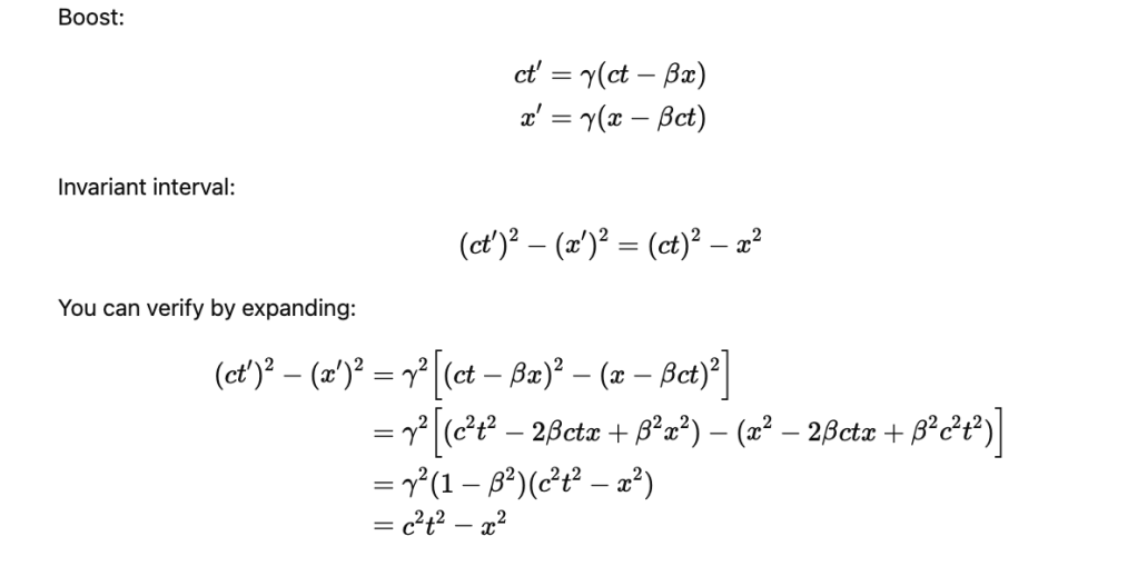
We can see that E/C and p transform the same way as ct and x above in order to arrive at our invariant (E/C)^2 – p^2

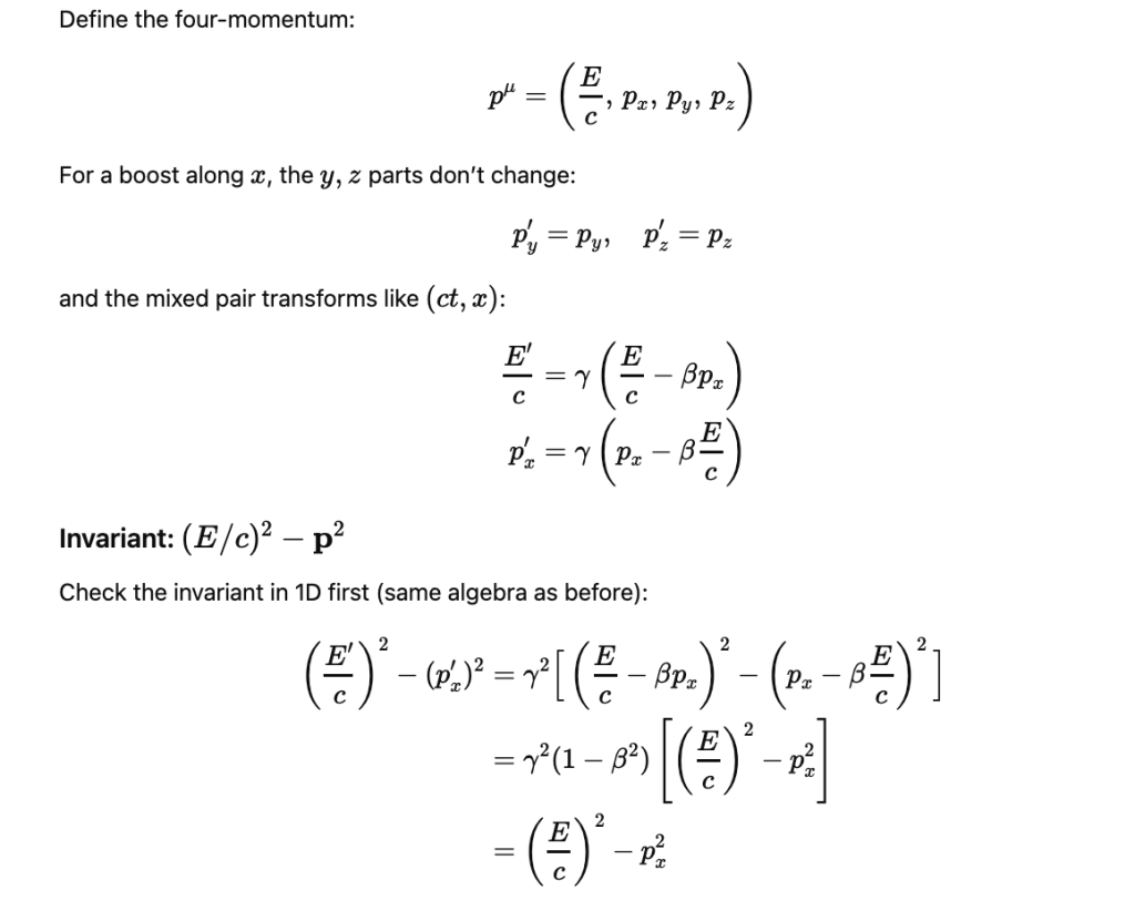
where $\beta = v/c$ and $\gamma = (1-\beta^2)^{-1/2}$ . This is the same result as when we contracted our covariant and contravariant components of p, which by necessity results in a scalar invariant.

Note that our 4 vector k transforms in exactly the same way as E/C and p because of the following:

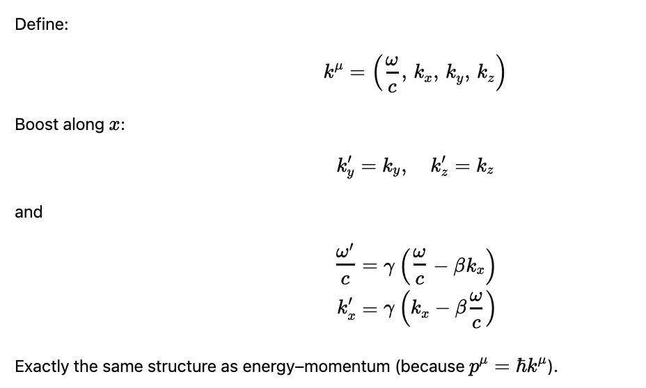
If you were to do the math, the k transform results into an invariant (w/c)^2 -k^2 , which can also be derived by the contraction of the covariant and contravariant components of k, which by necessity results in the scalar invariant above. This scalar means that no matter the frame in the same fashion as as the momentum transform results in our invariant (E/C)^2 -p^2.

Now, you want the same energy–frequency relation to hold in the primed frame. The only way for this to be consistent with Lorentz boosts is the following:

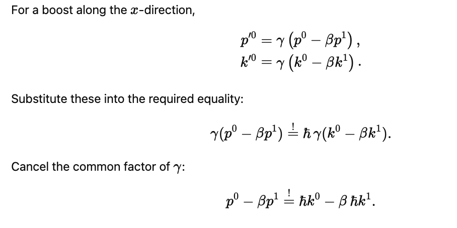
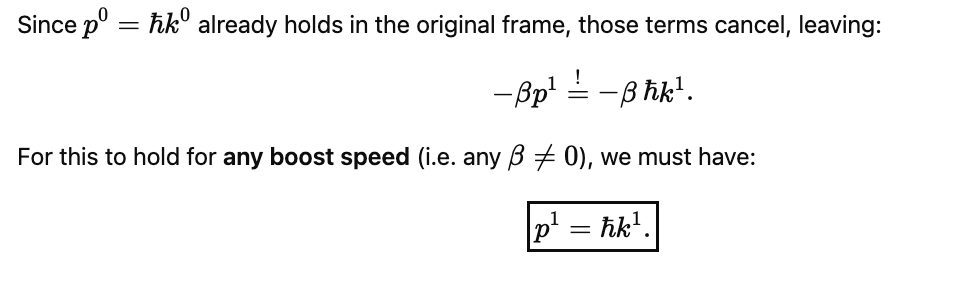
This would then be true for all the p and k components.

Rolling the Dice: A Derivation of Schrodinger’s Equation from the Wave Equation

Published by Josh Fialkow

Leave a comment Cancel reply

Share this:

Related

Published by Josh Fialkow

Leave a comment Cancel reply