
I wanted to examine two crucial principles in understanding the physics behind how systems flow- divergence and curl- and to fully explain both the mathematical assumptions and intuitions that underlie these bedrock foundations of field motion. I think what is most often overlooked in the explanations of divergence and curl is the fundamental importance in fully understanding the multivariable Taylor series expansion, and its concomitant assumptions that allow the proper derivation.
To begin to understand the concept of divergence, we must first examine flux. Flux tells us how strong a vector field is over a given surface. In the case of a fluid field, flux may tell us how many particles of the fluid are passing through a given surface per second. We can also apply flux to electric or magnetic fields, which would reveal the strength of the field through a surface rather than a velocity. To read more about the intuitions behind flux, please visit https://betterexplained.com/articles/flux/
Divergence uses the concept of flux to tell us how, at a given point, the field is operating as a source or a sink. If it is a source, more “stuff” (be it particles of fluid per second, strength of the electric field, etc) is leaving the point than entering and divergence is positive; if it is a sink, more “stuff” is entering the point than leaving and divergence is negative.
We can best understand divergence by first considering a two dimensional example. Below we have a square with its center point labeled and unit vectors extending upward from the midpoint of the top edge, 


 and horizontal side
Because we will be using a field filled with moving water as our example, let’s imagine that the water is moving upwards at great speed through the top edge. This movement would be represented by long upward pointing vectors anchored at the top edge extended upwards. At the bottom edge, let’s assume that there is still fluid moving upwards, just not as strongly as at the top edge, so we would represent this slower velocity with shorter vectors whose heads are touching the bottom edge and whose tails extend below that.
We can measure the flux through both of these boundaries by taking the dot product of the field vectors with the boundary’s normal vector, and then multiplying by 


We can begin to understand the concept of divergence by first asking: how can we compare the fluid flow between the bottom and top edges of the box?
There are six possible answers to this question if we assume that the fluid is flowing in the same direction. The first is based on our current example:
- Fluid is flowing up across both the bottom and top edges, but more fluid is flowing out of the top edge than is entering the bottom edge. Thus, relative to the center of the box, more fluid is leaving then entering, and we have positive divergence.
- Fluid is flowing up across the bottom and top edges, but more fluid is entering the bottom edge than leaving the top edge. Relative to the center of the box, more fluid is entering than leaving, and we have negative divergence.
- . Fluid is flowing down across the bottom and top edges, but more fluid is entering across the top than leaving across the bottom. Relative to the center of the box, more fluid is entering than leaving and we have negative divergence.
- Fluid is flowing down across the bottom and top edges, but more fluid is leaving across the bottom than entering from the top. Relative to the center of the box, more fluid is leaving than entering and we have positive divergence.
- and 6. Fluid is flowing up across both edges of the box at the same rate, or down across both edges at the same rate. In either case, we have 0 net divergence.
Of course, if the fluid field is not flowing in the same direction across top and bottom edges, we get even more possible combinations.
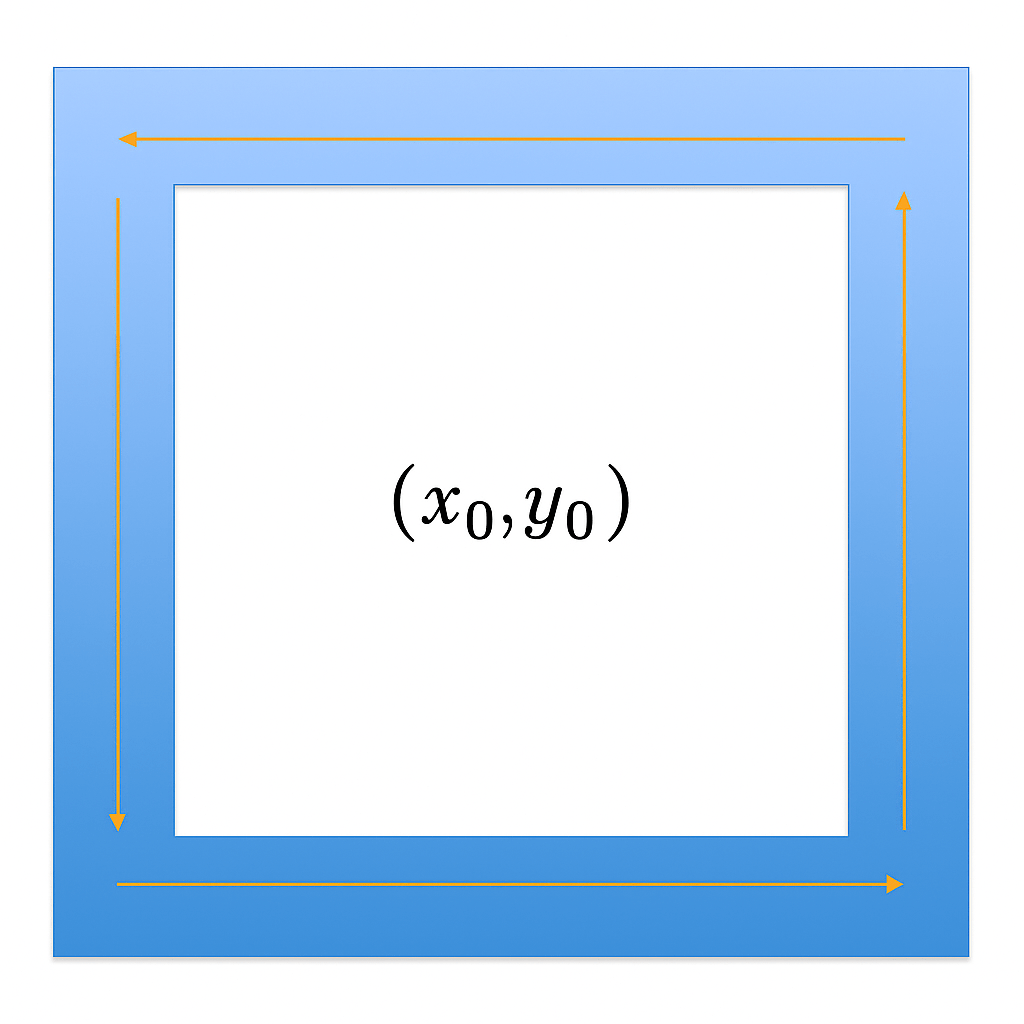
Divergence will seek to measure the change in the fluid flow right at a point. So let’s start to imagine shrinking the box as much as possible around its center point. If we shrink the box, we may get a better Taylor series estimate of the fluid field along the top edge by using the value of the field centered at the point F(xo,yo).
Because our function is centered in 2 dimensional space, we must account for the separate changes in the x and y variables. The general Taylor series estimate for a function of two variables centered at F(a,b) through the third derivatives is shown below:

Our (x-a) and (y-b) terms determine the steps we take from the center of the expansion, and thus represent a position vector with an independent x of component of length x-a and an independent y component of y-b. We will only be interested in going up to second derivatives (for reasons to be made clear later), so we can shorten the above expression to:

Note that the mixed derivative term would have a coefficient of 2 in front due to Clairut’s Theorem, but that 2 cancels due to the division by 2!. This is because though the mixed partial derivatives are equal to each other,

Below is a visual for why this must be true:
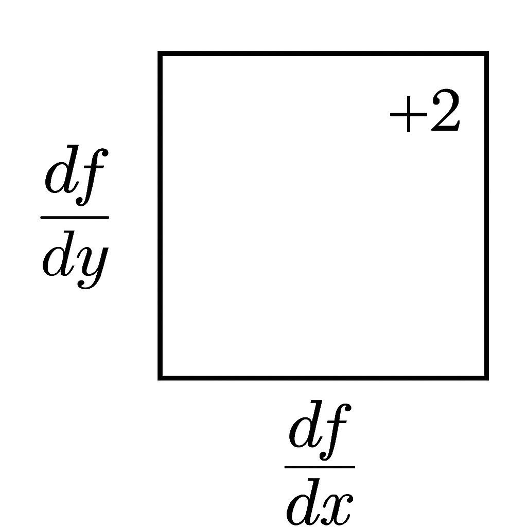
 Now we start again at the bottom left corner and take a single tiny step in the x direction and record df/dx. Then we slide up to see how df/dx changes and also record +2! This is exactly the meaning of
  These two expressions must be equal because we have to end up at the same spot in the top right corner, given that the function is smooth and continuous. Therefore, the change in df/dy and df/dx must be the same amount. This is also why we only want to count the mixed derivative one time: the function didn’t go up by +4, but only by +2 in total with respect to the second derivative as you travel from the bottom left to the top right (or along (x-a) and then (y-b), or vice versa. We can do this process to estimate how the first derivative changes along any given path, specified by the number of steps of x-a and y-b.
 To estimate the field function across the top edge of our box with the coordinates 


To estimate the field function across the bottom edge with the coordinates

Now we want to take the dot product of the vector field at the top edge with +j and then the vector field at the bottom edge with -j, and then integrate each separately by the x width of the box in order to obtain the net flux through the bottom and top boundaries. Here is the series of steps as a formula, before plugging in our Taylor approximation for the vector field:

Note that in the above formula, if the first expression is positive, it means the flux is leaving the top of the box ( and contributes to positive net flux) while if it is negative, it is entering through the top of the box (and contributes to negative net flux); in the second expression, if the flux vector is pointing in the same direction as -j, then the dot product is positive and it means that flux is leaving the bottom of the box (contributing to positive net flux) , while if the flux vector is pointing the the opposite direction as -j, then the dot product is negative and it means that flux is entering the top of the box (contributing to negative net flux). In practice, just the y component of the field vector would replace the dot product, since the y component of the field vector is exactly what the dot product of the entire field vector with the unit vector j actually is, so the integrals that follow will just show Fy , or y component of the vector field, rather than the entire dot product.
The brilliance of this simple formula is that it encapsulates the net contribution of all possible fluxes through the bottom and top of the box with a single number. If it is positive, we know more flux is leaving the box than entering, whereas if it is negative, we know more flux is entering the box than leaving. Of course, this encapsulates the net flux when fluid is flowing in the same direction, but it also does so when the fluid is flowing in different directions- for example if fluid is flowing down into the top of the box and up into the bottom, we would get 2 negative contributions and thus negative net flux.
Now we want to get a more precise definition of divergence using the Taylor series we already constructed. Let’s plug in our Taylor series estimates for the vector field inside each integral, and also take the negative sign in the second expression to the outside of the expression. The net flux across the x width of the box then can be shown to be the subtraction of integrals of the following dot products:
![\displaystyle \int_{x_0 - \frac{\Delta x}{2}}^{x_0 + \frac{\Delta x}{2}} \left[ F_y(x_0, y_0) + (x - x_0) \frac{\partial F_y}{\partial x}(x_0, y_0) + \frac{\Delta y}{2} \frac{\partial F_y}{\partial y}(x_0, y_0) + \frac{(x - x_0)^2}{2} \frac{\partial^2 F_y}{\partial x^2}(x_0, y_0) + (x - x_0)\frac{\Delta y}{2} \frac{\partial^2 F_y}{\partial x \partial y}(x_0, y_0) + \frac{1}{2} \left( \frac{\Delta y}{2} \right)^2 \frac{\partial^2 F_y}{\partial y^2}(x_0, y_0) \right] dx](https://s0.wp.com/latex.php?latex=%5Cdisplaystyle+%5Cint_%7Bx_0+-+%5Cfrac%7B%5CDelta+x%7D%7B2%7D%7D%5E%7Bx_0+%2B+%5Cfrac%7B%5CDelta+x%7D%7B2%7D%7D+%5Cleft%5B+F_y%28x_0%2C+y_0%29+%2B+%28x+-+x_0%29+%5Cfrac%7B%5Cpartial+F_y%7D%7B%5Cpartial+x%7D%28x_0%2C+y_0%29+%2B+%5Cfrac%7B%5CDelta+y%7D%7B2%7D+%5Cfrac%7B%5Cpartial+F_y%7D%7B%5Cpartial+y%7D%28x_0%2C+y_0%29+%2B+%5Cfrac%7B%28x+-+x_0%29%5E2%7D%7B2%7D+%5Cfrac%7B%5Cpartial%5E2+F_y%7D%7B%5Cpartial+x%5E2%7D%28x_0%2C+y_0%29+%2B+%28x+-+x_0%29%5Cfrac%7B%5CDelta+y%7D%7B2%7D+%5Cfrac%7B%5Cpartial%5E2+F_y%7D%7B%5Cpartial+x+%5Cpartial+y%7D%28x_0%2C+y_0%29+%2B+%5Cfrac%7B1%7D%7B2%7D+%5Cleft%28+%5Cfrac%7B%5CDelta+y%7D%7B2%7D+%5Cright%29%5E2+%5Cfrac%7B%5Cpartial%5E2+F_y%7D%7B%5Cpartial+y%5E2%7D%28x_0%2C+y_0%29+%5Cright%5D+dx&bg=eeeeee&fg=666666&s=0&c=20201002)
![\displaystyle -\int_{x_0 - \frac{\Delta x}{2}}^{x_0 + \frac{\Delta x}{2}} \left[ F_y(x_0, y_0) + (x - x_0) \frac{\partial F_y}{\partial x}(x_0, y_0) - \frac{\Delta y}{2} \frac{\partial F_y}{\partial y}(x_0, y_0) + \frac{(x - x_0)^2}{2} \frac{\partial^2 F_y}{\partial x^2}(x_0, y_0) - (x - x_0)\frac{\Delta y}{2} \frac{\partial^2 F_y}{\partial x \partial y}(x_0, y_0) + \frac{1}{2} \left( \frac{\Delta y}{2} \right)^2 \frac{\partial^2 F_y}{\partial y^2}(x_0, y_0) \right] dx](https://s0.wp.com/latex.php?latex=%5Cdisplaystyle+-%5Cint_%7Bx_0+-+%5Cfrac%7B%5CDelta+x%7D%7B2%7D%7D%5E%7Bx_0+%2B+%5Cfrac%7B%5CDelta+x%7D%7B2%7D%7D+%5Cleft%5B+F_y%28x_0%2C+y_0%29+%2B+%28x+-+x_0%29+%5Cfrac%7B%5Cpartial+F_y%7D%7B%5Cpartial+x%7D%28x_0%2C+y_0%29+-+%5Cfrac%7B%5CDelta+y%7D%7B2%7D+%5Cfrac%7B%5Cpartial+F_y%7D%7B%5Cpartial+y%7D%28x_0%2C+y_0%29+%2B+%5Cfrac%7B%28x+-+x_0%29%5E2%7D%7B2%7D+%5Cfrac%7B%5Cpartial%5E2+F_y%7D%7B%5Cpartial+x%5E2%7D%28x_0%2C+y_0%29+-+%28x+-+x_0%29%5Cfrac%7B%5CDelta+y%7D%7B2%7D+%5Cfrac%7B%5Cpartial%5E2+F_y%7D%7B%5Cpartial+x+%5Cpartial+y%7D%28x_0%2C+y_0%29+%2B+%5Cfrac%7B1%7D%7B2%7D+%5Cleft%28+%5Cfrac%7B%5CDelta+y%7D%7B2%7D+%5Cright%29%5E2+%5Cfrac%7B%5Cpartial%5E2+F_y%7D%7B%5Cpartial+y%5E2%7D%28x_0%2C+y_0%29+%5Cright%5D+dx&bg=eeeeee&fg=666666&s=0&c=20201002)
After subtracting the bottom expression from the top to capture the net flux across the bottom and top edges, many terms cancel out, leaving only the following relevant subtractions. First we subtract the third term in the bottom series from the third term in the top series:

and then the fifth term in the bottom series from the fifth term in the top series:

So the integral that is left is:
![\displaystyle \int_{x_0 - \frac{\Delta x}{2}}^{x_0 + \frac{\Delta x}{2}} \Delta y \left[ \frac{\partial F_y}{\partial y}(x_0, y_0) + (x - x_0) \frac{\partial^2 F_y}{\partial x \partial y}(x_0, y_0) \right] dx](https://s0.wp.com/latex.php?latex=%5Cdisplaystyle+%5Cint_%7Bx_0+-+%5Cfrac%7B%5CDelta+x%7D%7B2%7D%7D%5E%7Bx_0+%2B+%5Cfrac%7B%5CDelta+x%7D%7B2%7D%7D+%5CDelta+y+%5Cleft%5B+%5Cfrac%7B%5Cpartial+F_y%7D%7B%5Cpartial+y%7D%28x_0%2C+y_0%29+%2B+%28x+-+x_0%29+%5Cfrac%7B%5Cpartial%5E2+F_y%7D%7B%5Cpartial+x+%5Cpartial+y%7D%28x_0%2C+y_0%29+%5Cright%5D+dx&bg=eeeeee&fg=666666&s=0&c=20201002)
It is important to remember that the expression inside the integral above is only at the point xo,yo, which means that there are no x’s or y’s to integrate within the integral and we are just taking the integral of a number. After integrating, plugging in the bounds, and simplifying, we are only left with:

We are only left with the term above because the mixed derivative term is a constant, and when we integrate the term (x-xo) with the given bounds, we get 0! Each mixed derivative term (which is a constant) that is multiplied by (x-xo) to any odd power always equals 0 after integration.
Now we want to divide the above by 


By performing these operations, we get a nearly perfect approximation for the net flux around a point (area of 0), which is the very definition of divergence.
To summarize, after dividing our integral by 
This scalar number perfectly describes the overall net flux around a single point through our top and bottom edges, (or, equivalently put, the overall net flux at a single region whose area approaches zero). We now know that DFy/dy tells us the net flux, which is divergence, when considering flow through the bottom and top of the box, so we can conclude through the same exact method as above that DFx/dx tells us the divergence when considering the flow through the left and right of the box, and if adding a third dimension, DFz/dz would tell us the divergence when considering the flow in the z faces of a cube.
The formula for divergence is therefore just sum of the partial derivatives of the function and is expressed in 3d as:

This single number beautifully encapsulates how much the field at a given point’s location is behaving like a source or sink, with higher positive numbers indicating more source-like behavior, and lower negative numbers indicating more sink-like behavior.
Now let’s turn to the derivation of curl. Curl tells us how much field rotation there is around a given point. We create a box once again of area
For the bottom edge, when we walk in a positive x direction, and encounter a positive fluid field along that direction, we would get a positive counterclockwise flow contribution, but if we encountered a negative fluid field, we would get a negative clockwise flow contribution.
Taking the integrals of the dot product of the field with the negative i horizontal unit vector of the top horizontal edge plus the integral of the dot product of the field with the positive i horizontal unit vector of the bottom edge, we get:

Just like with divergence, the dot products reduce to just the relevant field component across the direction of motion, in this case Fx, the x component of the field vector, so we can rewrite the above expression as:

Now, we already know the Taylor series by which we can estimate the field along the top and bottom edges of the box from our previous discussion of the divergence theorem. We can generate our Taylor series in a similar fashiion; this time, instead of using the dot product, we will simply use the x component of the field vector in our series (which is equivalent to the dot product of the field in the direction of the horizontal i unit vector:
![\displaystyle -\int_{x_0 - \frac{\Delta x}{2}}^{x_0 + \frac{\Delta x}{2}} \left[ F_x(x_0, y_0) + (x - x_0) \frac{\partial F_x}{\partial x} + \frac{\Delta y}{2} \frac{\partial F_x}{\partial y} + \frac{1}{2}(x - x_0)^2 \frac{\partial^2 F_x}{\partial x^2} + (x - x_0)\frac{\Delta y}{2} \frac{\partial^2 F_x}{\partial x \partial y} + \frac{1}{8}(\Delta y)^2 \frac{\partial^2 F_x}{\partial y^2} \right] dx](https://s0.wp.com/latex.php?latex=%5Cdisplaystyle+-%5Cint_%7Bx_0+-+%5Cfrac%7B%5CDelta+x%7D%7B2%7D%7D%5E%7Bx_0+%2B+%5Cfrac%7B%5CDelta+x%7D%7B2%7D%7D+%5Cleft%5B+F_x%28x_0%2C+y_0%29+%2B+%28x+-+x_0%29+%5Cfrac%7B%5Cpartial+F_x%7D%7B%5Cpartial+x%7D+%2B+%5Cfrac%7B%5CDelta+y%7D%7B2%7D+%5Cfrac%7B%5Cpartial+F_x%7D%7B%5Cpartial+y%7D+%2B+%5Cfrac%7B1%7D%7B2%7D%28x+-+x_0%29%5E2+%5Cfrac%7B%5Cpartial%5E2+F_x%7D%7B%5Cpartial+x%5E2%7D+%2B+%28x+-+x_0%29%5Cfrac%7B%5CDelta+y%7D%7B2%7D+%5Cfrac%7B%5Cpartial%5E2+F_x%7D%7B%5Cpartial+x+%5Cpartial+y%7D+%2B+%5Cfrac%7B1%7D%7B8%7D%28%5CDelta+y%29%5E2+%5Cfrac%7B%5Cpartial%5E2+F_x%7D%7B%5Cpartial+y%5E2%7D+%5Cright%5D+dx+&bg=eeeeee&fg=666666&s=0&c=20201002)
![\displaystyle + \int_{x_0 - \frac{\Delta x}{2}}^{x_0 + \frac{\Delta x}{2}} \left[ F_x(x_0, y_0) + (x - x_0) \frac{\partial F_x}{\partial x} - \frac{\Delta y}{2} \frac{\partial F_x}{\partial y} + \frac{1}{2}(x - x_0)^2 \frac{\partial^2 F_x}{\partial x^2} - (x - x_0)\frac{\Delta y}{2} \frac{\partial^2 F_x}{\partial x \partial y} + \frac{1}{8}(\Delta y)^2 \frac{\partial^2 F_x}{\partial y^2} \right] dx](https://s0.wp.com/latex.php?latex=%5Cdisplaystyle+%2B+%5Cint_%7Bx_0+-+%5Cfrac%7B%5CDelta+x%7D%7B2%7D%7D%5E%7Bx_0+%2B+%5Cfrac%7B%5CDelta+x%7D%7B2%7D%7D+%5Cleft%5B+F_x%28x_0%2C+y_0%29+%2B+%28x+-+x_0%29+%5Cfrac%7B%5Cpartial+F_x%7D%7B%5Cpartial+x%7D+-+%5Cfrac%7B%5CDelta+y%7D%7B2%7D+%5Cfrac%7B%5Cpartial+F_x%7D%7B%5Cpartial+y%7D+%2B+%5Cfrac%7B1%7D%7B2%7D%28x+-+x_0%29%5E2+%5Cfrac%7B%5Cpartial%5E2+F_x%7D%7B%5Cpartial+x%5E2%7D+-+%28x+-+x_0%29%5Cfrac%7B%5CDelta+y%7D%7B2%7D+%5Cfrac%7B%5Cpartial%5E2+F_x%7D%7B%5Cpartial+x+%5Cpartial+y%7D+%2B+%5Cfrac%7B1%7D%7B8%7D%28%5CDelta+y%29%5E2+%5Cfrac%7B%5Cpartial%5E2+F_x%7D%7B%5Cpartial+y%5E2%7D+%5Cright%5D+dx+&bg=eeeeee&fg=666666&s=0&c=20201002)
For the same exact reasons when performing the integral sum to derive divergence, only one term ultimately survives after integrating the bounds up to the second order:

And, for the same reasoning as the divergence derivation, we first divide the expression by 


Now if we repeated this same process for the left and right edges, we would get the following terms, the first for the right hand side and the second for the left-hand side (for the left hand side, we have the dot product of the field with the negative vertical j unit vector, since we walk downwards along the left edge):


Plugging in the Taylor series estimate for the field vectors along each edge we get:
![\displaystyle \int_{y_0 - \frac{\Delta y}{2}}^{y_0 + \frac{\Delta y}{2}} \left[ F_y(x_0, y_0) + \frac{\Delta x}{2} \frac{\partial F_y}{\partial x} + (y - y_0) \frac{\partial F_y}{\partial y} + \frac{1}{8}(\Delta x)^2 \frac{\partial^2 F_y}{\partial x^2} + \frac{\Delta x}{2}(y - y_0) \frac{\partial^2 F_y}{\partial x \partial y} + \frac{1}{2}(y - y_0)^2 \frac{\partial^2 F_y}{\partial y^2} \right] dy](https://s0.wp.com/latex.php?latex=%5Cdisplaystyle+%5Cint_%7By_0+-+%5Cfrac%7B%5CDelta+y%7D%7B2%7D%7D%5E%7By_0+%2B+%5Cfrac%7B%5CDelta+y%7D%7B2%7D%7D+%5Cleft%5B+F_y%28x_0%2C+y_0%29+%2B+%5Cfrac%7B%5CDelta+x%7D%7B2%7D+%5Cfrac%7B%5Cpartial+F_y%7D%7B%5Cpartial+x%7D+%2B+%28y+-+y_0%29+%5Cfrac%7B%5Cpartial+F_y%7D%7B%5Cpartial+y%7D+%2B+%5Cfrac%7B1%7D%7B8%7D%28%5CDelta+x%29%5E2+%5Cfrac%7B%5Cpartial%5E2+F_y%7D%7B%5Cpartial+x%5E2%7D+%2B+%5Cfrac%7B%5CDelta+x%7D%7B2%7D%28y+-+y_0%29+%5Cfrac%7B%5Cpartial%5E2+F_y%7D%7B%5Cpartial+x+%5Cpartial+y%7D+%2B+%5Cfrac%7B1%7D%7B2%7D%28y+-+y_0%29%5E2+%5Cfrac%7B%5Cpartial%5E2+F_y%7D%7B%5Cpartial+y%5E2%7D+%5Cright%5D+dy+&bg=eeeeee&fg=666666&s=0&c=20201002)
![\displaystyle -\int_{y_0 - \frac{\Delta y}{2}}^{y_0 + \frac{\Delta y}{2}} \left[ F_y(x_0, y_0) - \frac{\Delta x}{2} \frac{\partial F_y}{\partial x} + (y - y_0) \frac{\partial F_y}{\partial y} + \frac{1}{8}(\Delta x)^2 \frac{\partial^2 F_y}{\partial x^2} - \frac{\Delta x}{2}(y - y_0) \frac{\partial^2 F_y}{\partial x \partial y} + \frac{1}{2}(y - y_0)^2 \frac{\partial^2 F_y}{\partial y^2} \right] dy](https://s0.wp.com/latex.php?latex=%5Cdisplaystyle+-%5Cint_%7By_0+-+%5Cfrac%7B%5CDelta+y%7D%7B2%7D%7D%5E%7By_0+%2B+%5Cfrac%7B%5CDelta+y%7D%7B2%7D%7D+%5Cleft%5B+F_y%28x_0%2C+y_0%29+-+%5Cfrac%7B%5CDelta+x%7D%7B2%7D+%5Cfrac%7B%5Cpartial+F_y%7D%7B%5Cpartial+x%7D+%2B+%28y+-+y_0%29+%5Cfrac%7B%5Cpartial+F_y%7D%7B%5Cpartial+y%7D+%2B+%5Cfrac%7B1%7D%7B8%7D%28%5CDelta+x%29%5E2+%5Cfrac%7B%5Cpartial%5E2+F_y%7D%7B%5Cpartial+x%5E2%7D+-+%5Cfrac%7B%5CDelta+x%7D%7B2%7D%28y+-+y_0%29+%5Cfrac%7B%5Cpartial%5E2+F_y%7D%7B%5Cpartial+x+%5Cpartial+y%7D+%2B+%5Cfrac%7B1%7D%7B2%7D%28y+-+y_0%29%5E2+%5Cfrac%7B%5Cpartial%5E2+F_y%7D%7B%5Cpartial+y%5E2%7D+%5Cright%5D+dy+&bg=eeeeee&fg=666666&s=0&c=20201002)
The only surviving term after integrating and plugging in the bounds is:

As we divide by
When we combine this result with the result of the rotation along the top and bottom edges, we find that our expression actually equals the cross product of the x and y components, which is a vector that points in the z direction:
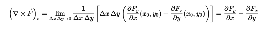
This checks out with our intuition. Let’s first examine what the positive dFy/dx term means. In the case where the y component of the field is positive, a positive dFy/dx means that as we take an infinitesimal step in the positive x direction around a point, we must have more push up on the right side of the point than on the left side, thereby resulting in positive counterclockwise rotation; in the case where the y component of the field is negative across both the left and right vertical edges, a positive dFy/dx term means we have more push down on the left side of the point than on the right side, thereby also resulting in positive counterclockwise rotation. For the last possibility, a positive dFy/dx can indicate the y component of the field changing from a negative to a positive number as we take a small infinitesimal step dx, which also results in a positive counterclockwise flow since both the negative flow downwards along the left side and a positive flow upwards along the right side both contribute to positive counterclockwise flow.
Now let’s get the intuition for why -dFx/dy contains a negative sign in front by considering why when dFx/dy itself is positive, we must add a negative sign in front of it to signify negative clockwise flow. Let’s assume that the x component of the field is positive, and is increasing as we take a small step dy up: this translates to stronger flow rightwards across the top edge than rightwards across the bottom edge, thereby resulting in a negative clockwise flow (which is why the negative sign must appear outside a positive dFx/dy). If the x component of the field is negative along both edges, a positive dFx/dy means that it is less negative along the top edge than along the bottom edge, so the negative leftwards push along the bottom edge dominates and we get a net negative clockwise flow. The final reason why dFx/dy may be positive is if the x component of the flow is negative (leftwards flowing) on the bottom edge and positive (rightwards flowing) on the the top edge, in which case we get both edges contributing to clockwise motion and we must place a negative sign in front of the positive dFx/dy. So in all 3 cases, a positive dFx/dy indicates clockwise flow and we must place a negative sign in front; if dFx/dy is negative, we get positive counterclockwise flow and need the negative in front in order to make the dFx/dy positive!
The full expression for curl in three dimensions is:

In the zy plane, z is a vertical edge and y is a horizontal edge; in the xz plane, x is a vertical edge and y is a horizontal edge, and of course, in the yx plane, y is the vertical edge and x is the horizontal edge. But what if in the yx plane, for instance, we viewed the y’s as our horizontal edges and the x’s as our vertical edges due to a rotation? You would actually still get the same exact value for curl if you rotated each plane 90 degrees clockwise. For example, if you rotated the xy plane 90 degrees clockwise, now x would be the vertical edge and y would be the horizontal, and we would calculate (dFx/dy – dFy/dx) instead of (dFy/dx – dFx/dy). But switching the order would still preserve the value of the curl. If when x was horizontal, dFx/dy was positive (for example, with the top edge experiencing a stronger flow rightwards than the bottom edge), we know that this would contribute to a negative clockwise rotation so we would have originally subtracted this positive dFx/dy value. However, after rotating the plane 90 degrees clockwise so that x was now on the vertical edges and y on the horizontal edges, we would now find that dFx/dy would be negative already (with the right edge showing a stronger downward flow than the left edge), correctly indicating clockwise contribution. So, we would no longer need the negative sign in front of dFx/dy. Now, however, we would need the negative in front of the dFy/dx term instead to correct for its contribution, which exactly what the new order of (dFx/dy – dFy/dx_) does! So by rotating the plane by 90 degrees, we do not affect the value in the parentheses. This agrees with the concept that you still get the same vector even if you rotate the frame.
The discussion of the curl as a cross product links to our previous discussion about cross products at https://mathintuitions.com/2022/09/30/geometrical-proof-of-the-cross-product/ . Below is a chart that connects the algebraic discussion in our previous post on the cross product with the curl expression derived in this post:

And here are the relevant formulas and expressions:

I hope that this discussion has been a valuable tool into fully understanding where the formulae of divergence and curl come from, with intuitive yet rigorous understandings of the multivariable Taylor series and physical meanings of the formulas.
