
The aim of this two-part post is to fully derive and compare the paths of planetary orbits in classical Newtonian physics and Einstein’s General Relativity. Though the two versions are similar in describing planetary elliptical orbits, the General Relativity version accounts fully for the precession of the elliptical paths, which means that the elliptical paths actually rotate as shown in the image below (the Newtonian version accounts for this precession too, but just not as accurately as the General Relativity version):
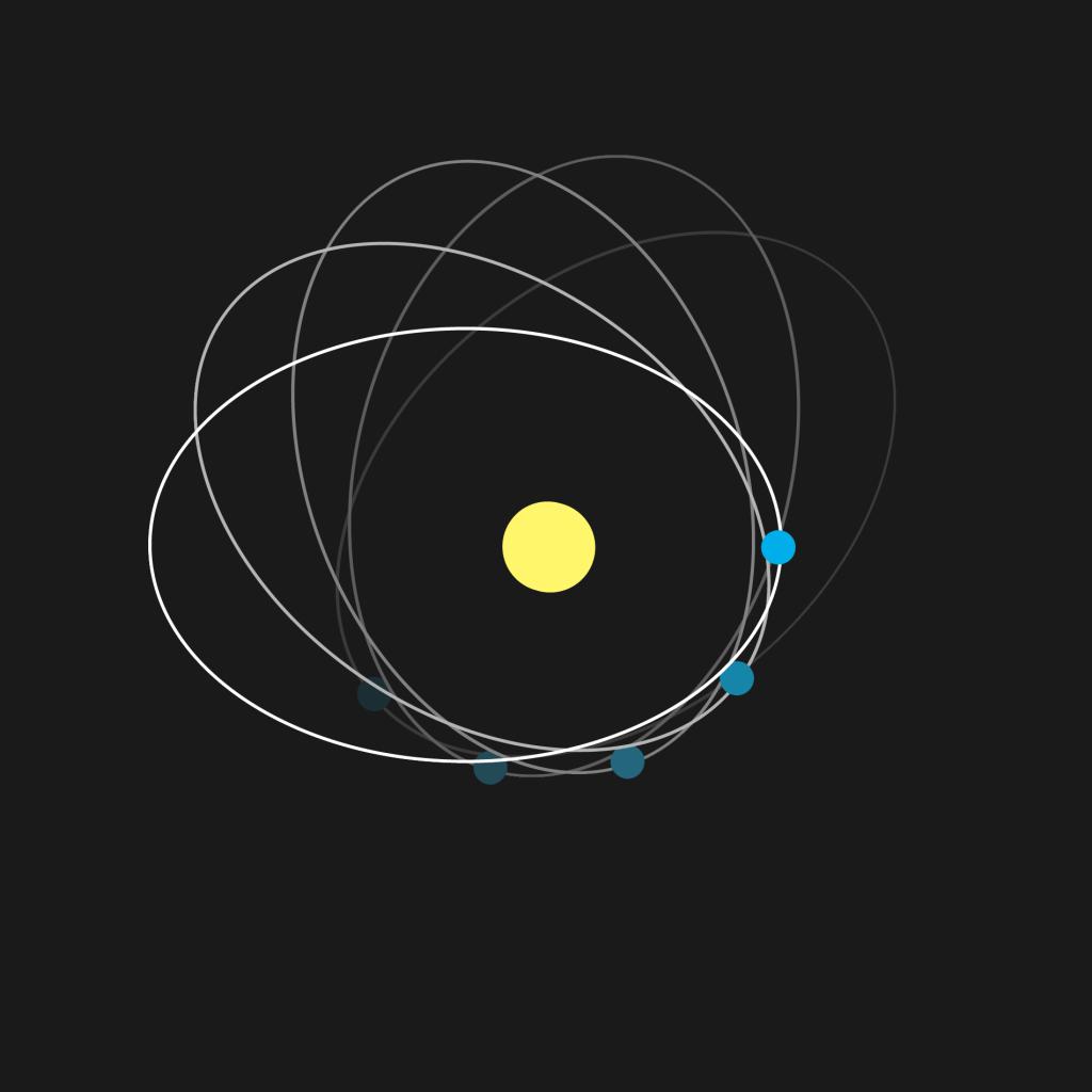
from https://en.wikipedia.org/wiki/Tests_of_general_relativity#/media/File:Apsidendrehung.png
Many mathematical techniques and assumptions involved in these derivations will be fully explained, which will help to understand each step. Additionally, we will strive to derive the orbital paths in both classical and relativistic models in such a way as to most easily compare the end results, for which authors often create different forms that are difficult to compare. This post, Part I, will derive the Newtonian classical orbital paths to make them most comparable to those presented in General Relativity.
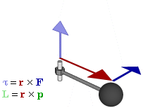
In physics, any object that is moving in a circular path without any external force perpendicular to the “lever arm” (known as the torque) will conserve its angular momentum. This is valid for planets in orbit as well. As we will see, planets have 0 torque, which means they have no external force applied in a perpendicular fashion to their orbital radius; since these orbital paths have 0 torque, the planets’ angular momentum is constant. Although all orbiting planets do have a gravitational force, this force acts parallel to the orbital radius rather than perpendicular to it and thus the torque is still 0.
Below is a case where the net torque, shown as the cross product of the radial lever arm and the applied force, is positive (torque= r x F).

from https://upload.wikimedia.org/wikipedia/commons/0/09/Torque_animation.gif
However, as previously stated, a planet that is orbiting the sun or any other body has zero net torque, since the gravitational force acts parallel to the radial lever arm resulting in a cross product of 0. For more clarity on cross products, please go to a previous post at https://mathintuitions.com/2022/09/30/geometrical-proof-of-the-cross-product/
Now to see why a 0 net torque results in a constant angular momentum (shown in the image above as the cross product of L= rxmv=rxp) of the planet, we first convert Newton’s law F=ma to its appropriate analogue for circular motion by taking the cross product of each side with respect to the radial lever arm:
rxF = rxma
If we know that the torque, rxF, of the left-hand side is zero, this would mean that (r)x(ma) is also 0. As we know, acceleration is the derivative of velocity, so we can rewrite rxma=0 as d(rxmv)/dt=0 (we can also take the derivative of the radius along with the velocity term since the dr/dt term crossed with velocity will be 0 anyway, as we will see). Now, applying the product rule, d(rxmv)/dt equals (dr/dt)x(mv) +(r)x(ma). The dr/dt term is equivalent and parallel to v, the velocity (which equivalently shows how the radius changes its position over time), so the cross product of (dr/dt)x(mv)=0 as previously stated. So what we have performed is summarized by the following equation:
0=rxF=rxma= d(rxmv)/dt= (dr/dt)x (mv) + (r)x(ma)= 0 +0.
The term (r)x(mv) is the angular momentum, and is often written as rxp, where p=mv. Since we just proved that the derivative of this angular momentum term is zero for orbiting planets due to a 0 net torque, this means that the angular momentum must be constant, or conserved. We will relabel this constant term of angular momentum as L.
Now we can begin to fully derive the planetary orbital equations under Newton’s and Einstein’s models. There are two amazing videos that derive each: for the Newtonian model it is https://www.youtube.com/watch?v=wLYZsO6lk0E. For the General Relativity Model, it is https://www.youtube.com/watch?v=up4p-s7x56g.
Both videos do a much better job than I could, though they omit some mathematical steps and also present different forms for the orbital paths in the Newtonian model, which only the first video derives.
So, we will first attempt to derive the orbital paths in the Newtonian model that will have a form more directly comparable to the form typically presented in General Relativity. We begin our derivation with the previously recognized fact that the angular momentum L of a planet’s orbit is constant and that our gravitational force, derived in a previous post at https://mathintuitions.com/2023/06/23/a-mystery-with-gravity-the-gravitational-constant-g-derived-from-newtonian-principles/, is:
The easiest coordinate system to use in order to model circular motion is polar coordinates, or in the case of 3 dimensions, spherical coordinates.
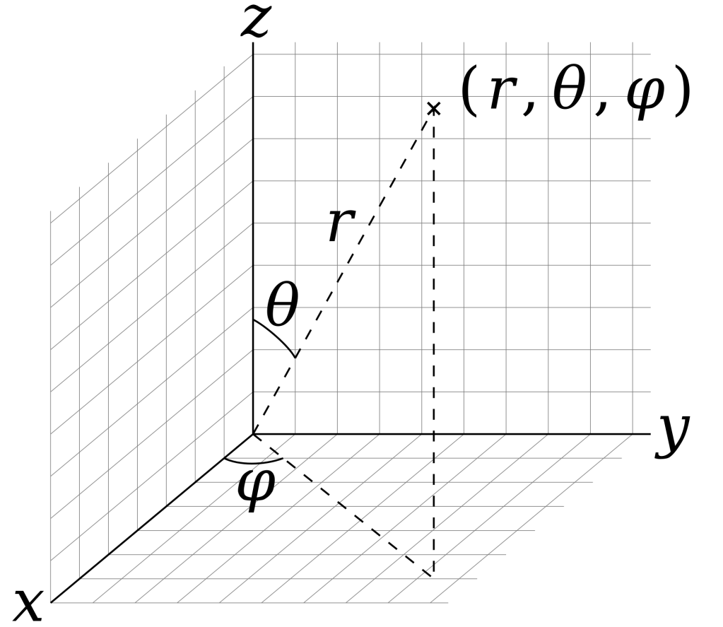
from https://en.wikipedia.org/wiki/Spherical_coordinate_system#/media/File:3D_Spherical.svg
We are striving to understand how the planet’s radial position, r, is a function of its angle, phi., to the star that it orbits. You may notice that using r and phi only results in 2 dimensions whereas the world in which we live in consists of the 3 spatial dimensions as shown in the image above. The reason why we can use just r and phi is because we can assume that theta (the angle made between the z axis and r shown above) is constant at 90 degrees in the equatorial plane, since we can always rotate our coordinate system to make this true of the orbital path.
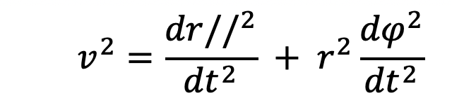
Now that we have covered some basics about the coordinate system and angular momentum, we can start to model the orbital path of a planet. In the image below we see a planet with a velocity v=dr/dt, broken down into 2 components: the velocity component perpendicular to the radius is r(dphi/dt) and the parallel component to the radius is ((dr//) / (dt)).

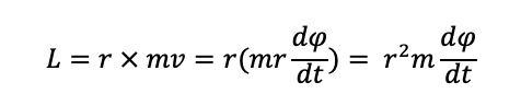
The angular momentum of the object above is given below, which shows the cross product of the radius and massxvelocity, which means this calculation only involves the perpendicular component of the velocity and not the parallel component of the velocity:
We also know that the total energy in this system = kinetic energy + potential energy + rotational energy (which will be neglected since it is dwarfed by the other terms), and so we have
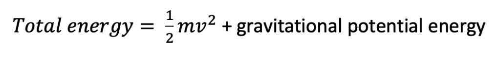
where 1/2mv^2 is the kinetic energy term.
We can break down the 1/2mv2 into both the perpendicular and parallel components of velocity, since the magnitude of the square of the velocity vector is:
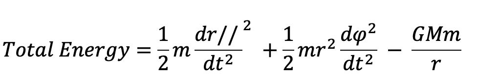
Also, the gravitational potential energy term is -GMm/r, whose derivation can be found at http://hyperphysics.phy-astr.gsu.edu/hbase/gpot.html
So if we substitute in the components for v^2 and the for gravitation potential energy term in our total energy equation, we get:
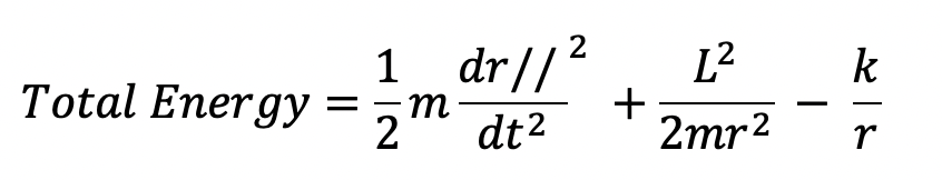
We can algebraically manipulate the second term by multiplying numerator and denominator by r^2/m in order to express it more simply:

which gives us the advantage of using the constant L such that the second term is really only dependent on r, assuming a constant mass.
We can also simplify the gravitational potential term with a constant k=GMm. k is only dependent on the gravitational constant G and the two masses of the objects which we take as constants as well. So L and k both don’t change. With these constants employed in the total energy equation, we now get that total energy is equal to
I am now going to drop the parallel lines in the dr// / dt term. It will still refer to radial velocity, which is parallel to the radius itself, rather than the overall velocity.
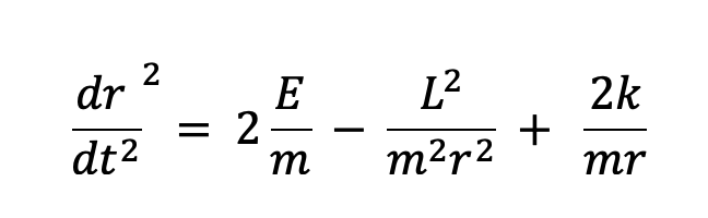
We can solve for this (dr/dt)^2 now in terms of the other variables through some algebraic manipulation, where E is the total energy:
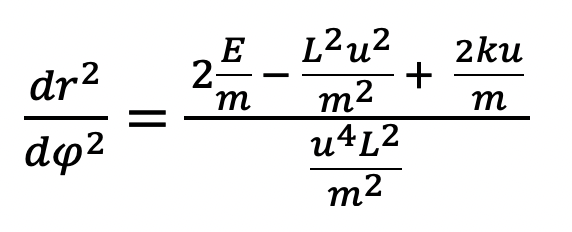
Now, our goal is to get how the radial position changes as a function of phi (remember, the dr/dt term shows us how the radial length is lengthening or contracting over time ). Our next step to accomplish this is to solve for (dphi/dt)^2 in our angular momentum term, and then to divide (dr/dt)^2 by (dphi/dt)^2 to get (dr/dphi)^2:
Starting with our angular momentum equation:

we can solve for (dphi/dt)^2 :

Then, we divide our already known expression for (dr/dt)^2 by (dphi/dt)^2 to get the term we are interested in, (dr/dphi)^2:

At this point, this derivation of planetary orbits under classical physics will diverge with the derivation presented at https://www.youtube.com/watch?v=wLYZsO6lk0E in order to get a more comparable formula to orbits formulated under general relativity. The divergence occurs based on a different substitution: we will instead substitute “u” for “1/r” and get the following:
Because the above shows that an expression exists for dr/dphi, that must mean that r, the radial coordinate, can be expressed as a function of phi.
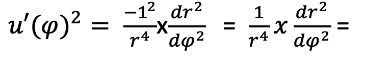
Now given that we have defined “u” to be “1/r’, it follows that

We will also assume that u and its derivative u’ are functions of phi, since u is a function of r and r is a function of phi so :

Again, the dr term refers to the infinitesimal change parallel along the radial coordinate, which signifies the contracting or lengthening of the radial position, whereas dphi is the change in the direction perpendicular to the radial length.
The next part of our derivation is also omitted from the video derivation and just involves a lot of substitutions and algebra to arrive at our final expression for u'(phi)^2. We plug in our expression for du/dr and substitute:
Then we plug in our previously derived expression for (dr/dphi)^2:
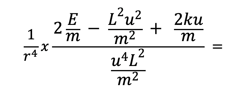
Next, we take the denominator and distribute it to each of the three terms in the numerator :

and then we simplify by cancelling some of the m’s, u’s and L’s:
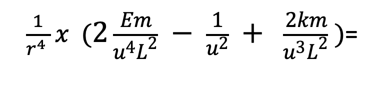
After simplifying, we can substitute u^4 for 1/r^4:
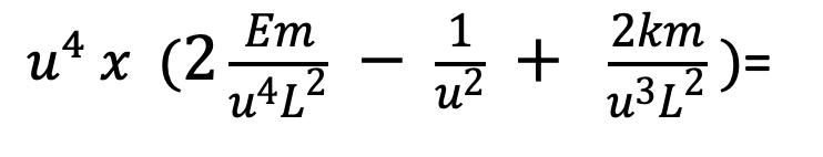
and then distribute the u^4 to each term, and simplify by cancelling the u’s in order to obtain our final expression for u'(phi)^2:

Now to figure out what u(phi) is, we need to take the derivative again with respect to phi in order to relate u’ to u”; this relationship will make the value of the original function u clearer;
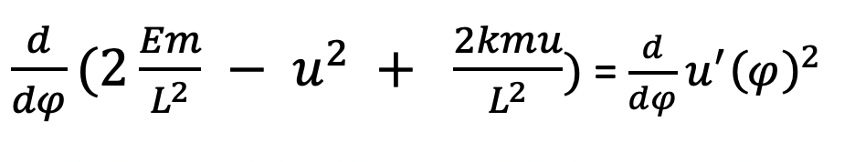
To compute the derivative with respect to phi, we utilize the chain rule for the u^2 and u’^2 functions in the above equations, as well as take a simple derivative of u in the 2kmu/L^2 term. For example, with the u^2 term, we must perform d(u^2)/du x (du/dphi)= 2uxu’, where u’= du/dphi; for the u’^2 term, the derivative with respect to phi would also use the chain rule to get 2u’xu”. The expressions 2uxu’ and 2u’xu” thus give the derivatives of u^2 and u’^2 with respect to phi. Moreover, the constant 2EM/L^2 drops out of the derivative since it does not contain any functions in terms of phi, so the full equation becomes:
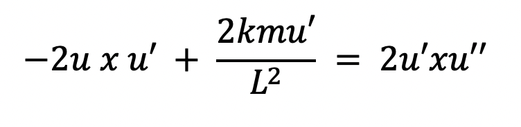
Dividing each side by u’ and 2 we get the simpler expression (and one that will be more useful to compare with that in general relativity):
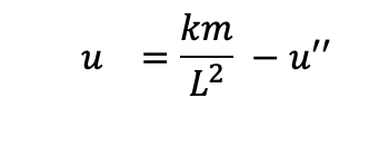
If we isolate the u term, we get the following:
The question then becomes: what function and its second derivative are essentially the same, but just opposite signs? The answer is clear: either ( or both of) the sin or cos function. We will go with the cos function (it doesn’t really matter which one we choose, since we can express one as a phase shift of the other). The first derivative of (cosine) is (- sine), and the second derivative of (cosine) is thus (- cosine). It is important to note that this relationship would hold for any number times cosine, so for example, the first derivate of 5x(cosine) is -5x(sine), and the second derivative would be -5x(cosine). Because we are not sure what number is multiplying our cosine function, we will say that our original function is Ex(cosine), the first derivative is -Ex(sine) and the second derivative is -Ex(cosine), where the E is an unknown number in our notation (for a more full understanding of how to solve this second order differential equation, go to https://www.mathsisfun.com/calculus/differential-equations-second-order.html , where we find that Asin + Bcos can be combined with a phase shift in the cosine term).
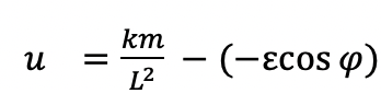
So we have determined that u” = -Ex(cosine)
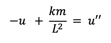
It is clear that the km/L^2 term disappears for the second derivative of u with respect to phi, denoted by u”(phi), since the km/L^2 term is a constant and has no phi in it. So if u” is (-E x cosine) as we previously established, that would mean that u itself would equal the following:
And after simplifying and rearranging:

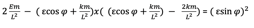
Now we have to figure out the number E that must be multiplying the cosine(phi) term. To nail down what the number E is, we go back to our equation for u'(phi)^2:
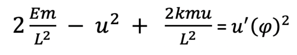
Next we plug in the following expressions for u and u’
and du/dphi, or u’, would thus be u’= – (Exsin), so:

Taking out the common factor of Ecos(phi) + km/L^2 on the left side and removing the negative from the right side since it is a squared term results in:
We can then subtract -2km/L^2 from km/L^2 and get:

The middle two terms are the difference of 2 squares, so we can further simplify (a +b)(a-b) = a^2 – b^2, where a= Ecosphi and b=km/L^2:

and distributing the negative;

Moving the -Ecos(phi)^2 to the other side, we find:
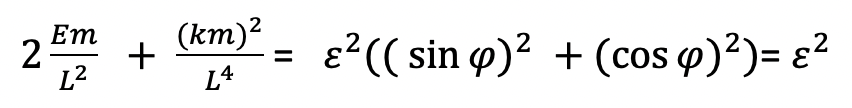
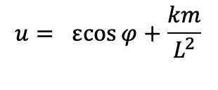
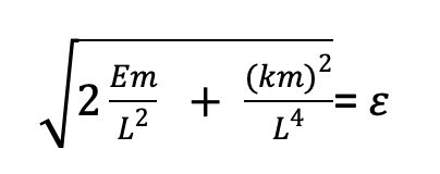
So E (the squared number on the right) must equal, (whereas the E in the Em term is the energy):
Thus, our equation for “u” which was

becomes with the substitution for the term multiplying cos(phi):
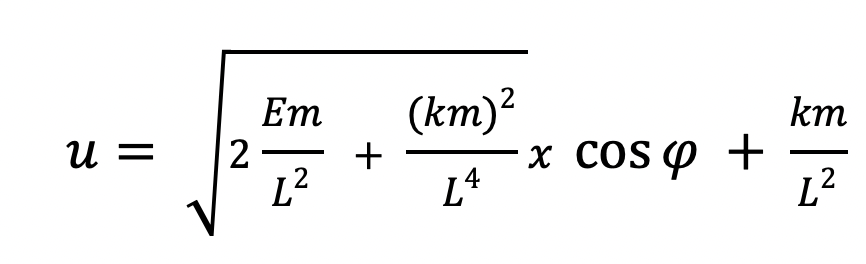
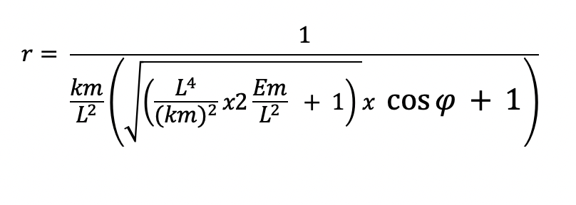
Since we defined u=1/r, then r=1/u. Plugging in our expression for u, we find that:

Note that this gives r as a function of the angular variable phi, which was out desired goal; the other terms are constants.
Our next question is, what kind of shape is this strange looking equation? How can we possibly make sense of this?
Through some algebraic manipulation, we can arrive at the fact that this big mess is actually the equation for an ellipse:
We are going to insert the term

, which equals 1, in the square root in the following manner:

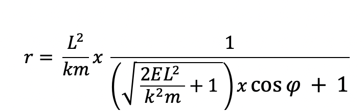
Here the (km)^2/L^4 is a common factor to both the 2Em/L^2 term and itself ; in the end, we have only multiplied the 2Em/L^2 term by 1 and thus have left the original equation unchanged.
Now we can take the square root of the common factor (km)^2/L^4 and move it outside the square root sign: and factor
and further simplify by cancelling L’s and m’s in the L^4/(km)^2 x 2Em/L^2 terms under the square root and put
L^2 in the numerator:

Then we can just take the L^2/km term as its own separate term multiplying the rest:

This is actually the equation of an ellipse! To see why, let’s derive the equation of an ellipse through the following diagram:

Now we know that the eccentricity, e, of any conic section can be defined as the ratio of the distance from the focus to the point on the conic divided by the distance of the point on the conic to the directrix (the previous post on parabolas at https://mathintuitions.com/2024/02/16/to-infinity-and-beyond-the-parabola-as-an-infinite-ellipse/ makes it clear as to why the eccentricity can be defined in this manner).
Based on this definition of e, the above diagram shows that e would equal r/D. Therefore, if we solve for r, we get
r= eD
We can see from the diagram that D also equals D= (d – rcos(phi)).
Substituting this expression for D in r=eD, we get that : r = e(d-rcos(phi))= ed – ercos(phi).
Let’s move the last term over to the left side and then factor out the “r” term to obtain: r(ecos(phi) + 1)= ed.
Now let’s divide by the (ecos(phi) + 1) term on each side to get our expression for r:
r= ed/(ecos(phi) + 1). Notice that this form exactly :
where e, the eccentricity of Earth’s orbit, is the term multiplying cos(phi): e=
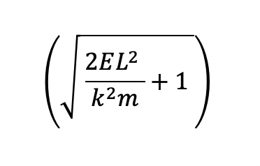
and the “ed” term in r= ed/(ecos(phi) + 1)would be L^2/km. Earth’s eccentricity is accepted at or near the value of .0167, which is what we find in the following calculation using numbers for energy, angular momentum, and values for “k” including gravitational constant, and the masses of the Earth and the sun:

This value of .0167, an elliptical eccentricity very close to a circle’s value of 0, is typically found by looking at physical observations of the ellipse that Earth makes, rather than using the extremely large and small values for energy, angular momentum, gravitational constant and masses of the Earth and Sun. One issue with the above calculation is that to obtain the accepted eccentricity value of .0167, I had to very slightly alter some of the accepted numeric values for energy , angular momentum etc., since any tiny changes in these extremely large and small numbers results in wildly different values for the eccentricity. The numbers obtained from Earth’s planetary fact sheet (found in the appendix of https://mail.wbabin.net/Science-Journals/Research%20Papers-Astrophysics/Download/7533) for energy, angular momentum and mass do not in fact result in the given eccentricity for Earth’s orbit (probably due to the fact that the tail end of these giant numbers are approximated), which means that either the numbers that are commonly used for energy, momentum, etc. are not completely correct or Earth’s commonly accepted eccentricity is not completely correct. But it’s interesting to me how most reference sheets list these numbers along with Earth’s planetary eccentricity (in Newtonian form) without realizing that those numbers are not correctly adding up in the equation!
Now that we have properly established how a planet’s orbital position in Newtonian physics is a function of its angle given by :
we can proceed to the next post that will derive this elliptical relationship under the assumptions of general relativity, which will expand upon the Newtonian form by showing that the elliptical orbital paths actually rotate, given the mathematics behind the equation!
