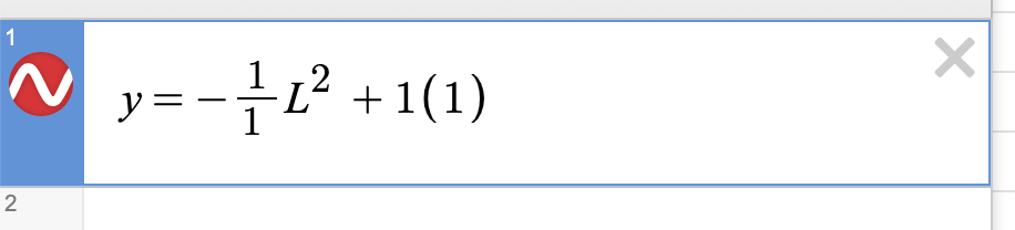
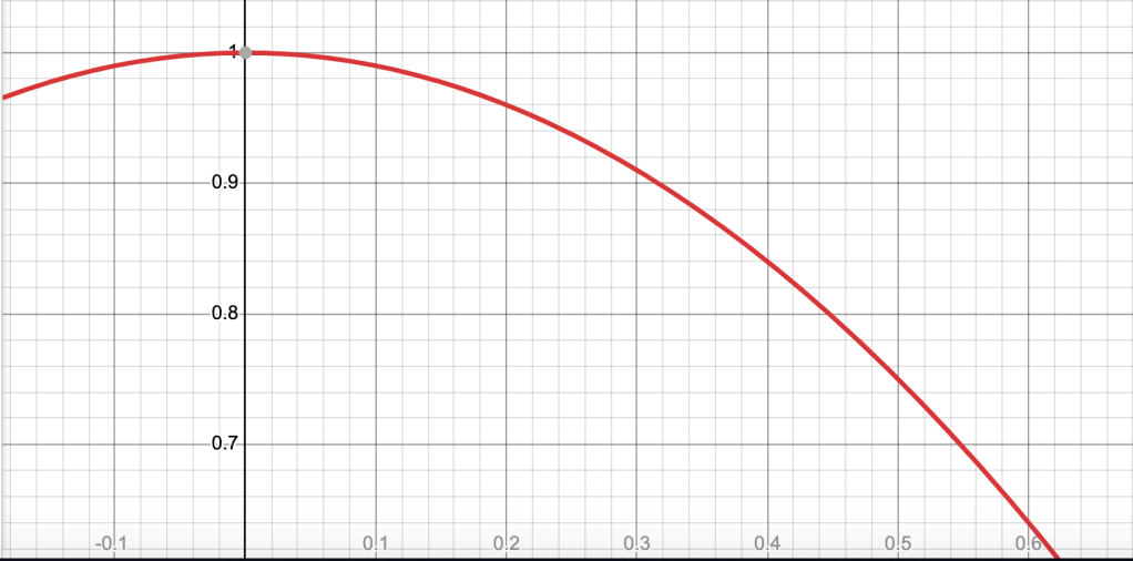
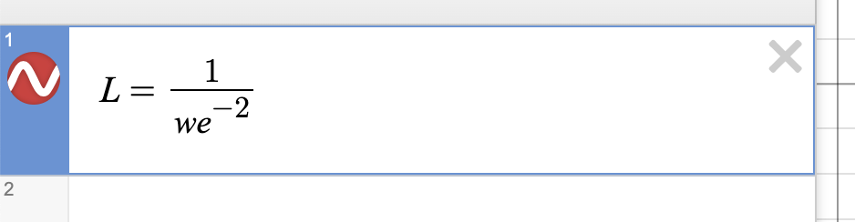
In our previous post, we found that area cannot be maintained through equal but opposite percent changes in length and width using algebraic techniques. We determined that when we increased length by a certain percentage and decreased width by the same percentage, our new area calculation was derived through a downward sloping parabola of the form:

As a visualization of the above equation, we assumed we started with a rectangle of length= 1 and width=1 whose area was therefore 1. We showed that when we increased the length by 30% and decreased the width by 30%, the new area was .91, or a 9% decrease of the original area. The x variable, shown below, represented our percent increase of length and percent decrease in width with original length and width chosen as 1.
The fundamental error in assuming that our equal yet opposite percent changes in our length and width variables could preserve area concerns the following intuition: we were assuming that our original length and width variables were not changing, even though in fact they were constantly changing! This nature of constant change implies we need more advanced mathematics than algebra; namely , we must utilize calculus, which best models the world of constantly changing quantities.
As a more concrete understanding of the above intuition, let’s take a representative case with simple numbers. Starting with the number 100, if I apply a 1 % increase, I get 101. If I increase 101 by 1% again, I get 102.01; however, if kept 100 as constant and applied a 1% change to 100 and added another 1% change to 100 (in other words, increasing 100 by 2%), then I only get 102 rather than 102.01. So we must take into account that for every infinitesimal percent increase and decrease we apply to our length and width dimensions, we change our original variables of L and W that were incorrectly assumed to be static constants in the equation

Because length and width constantly change given percent changes, we decided we are likely to need calculus, or the mathematics of change, to deal with keeping area constant. We also are likely to deal with the number e, which helps us understand how a number grows or decays after infinite compounding, where for example we get 102.01 instead of 102 as shown above.
Question: How do we create an equation that maintains constant area using equal percent changes in length and width?
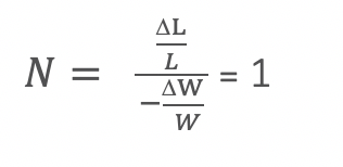
Let N= the factor by which area changes.
Now we want N to equal 1 so that our area doesn’t change.
We also assumed that L and W changed by equal but opposite percentages so:
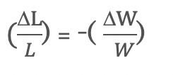
Now the factor N is the factor by which area changes. It can be seen as the percent change in L divided by the percent change in W. If the numerator is much greater than the denominator, that would mean that a small percent decrease in width would cause a large percent increase in length, thus resulting in a factor for N greater than 1 which would increase the area. On the other hand, if the numerator is much smaller than the denominator, that would mean that the percent decrease in width far outweighed the percent increase in length, and N would be less than 1 which would decrease the area. However, we would like N to be 1 to maintain a constant area, so we would have:
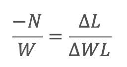
After cross multiplying and then dividing by ∆W, we get
Now comes a crucial leap of faith: let’s assume our length variable, L, can be written as a function of our width variable, W. So we have L{w} as a function. This function can truly be any linear or curvilinear relationship you want before plugging the L{w} equation into the constraint of the equation.
It makes sense that L would be a function of W because as we take infinitesimally equal yet opposite percentage changes for each variable with our constraint in the equation, we will smoothly run through all the numbers in the number line. Our mission is to find out the precise relationship between L and W to keep area constant.
Because of our assumption that L is a function of W, the derivative of the L{w} function is
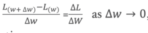
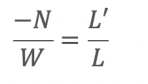
we can substitute L’ , symbolizing the derivative of L, for

on the right hand side of the equation:

Rewriting the above proportion with said substitution, we obtain:
Next, let’s integrate both sides of this equation with respect to the variable W to “get rid of” the derivative. Keep in mind, the right side of the equation can be written in terms of the variable W, since we’ve assumed that L is a function of W:
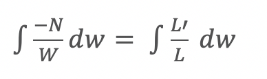
So after integration, we get:
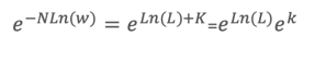
-NlnW=ln(L)+K
where k is the constant of integration, which as we will see represents whatever the area is that we want to maintain as a constant.
Now we raise both sides to e to obtain:
This equation then leads to:
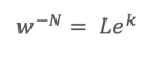
Dividing each side by

we obtain :
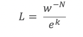
To maintain constant area, N, or the factor by which we multiply the area, must equal 1:
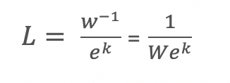
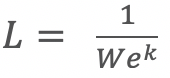
So to keep area constant, the relationship between our length and width values is given by the above equation. Using e means that we are subjecting our length and width dimensions to infinite compounding and readjusting the original constant values as needed.
If we multiply both sides of the equation by W, then we get
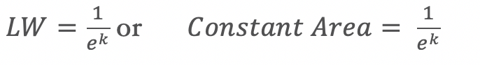
We have thereby derived an equation for maintaining constant area of a rectangle by using infinitesimally equal yet opposite percent changes in our length and width variables. It is evident that k determines whatever the area number is that we want to keep from the above equation.
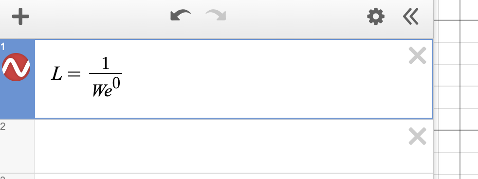
If we want the area to be maintained at a constant of 1, then we solve for k:
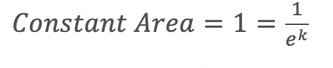
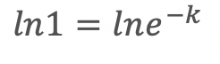
Given the above equation, k must equal 0 to maintain a constant area of 1.
Next, plug in 0 for k in the equation to get the relationship between length and width to keep area constant at 1 :
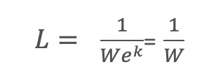
Which makes intuitive sense since by multiplying a number by its reciprocal you always get 1, which is the constant area we wanted to maintain.
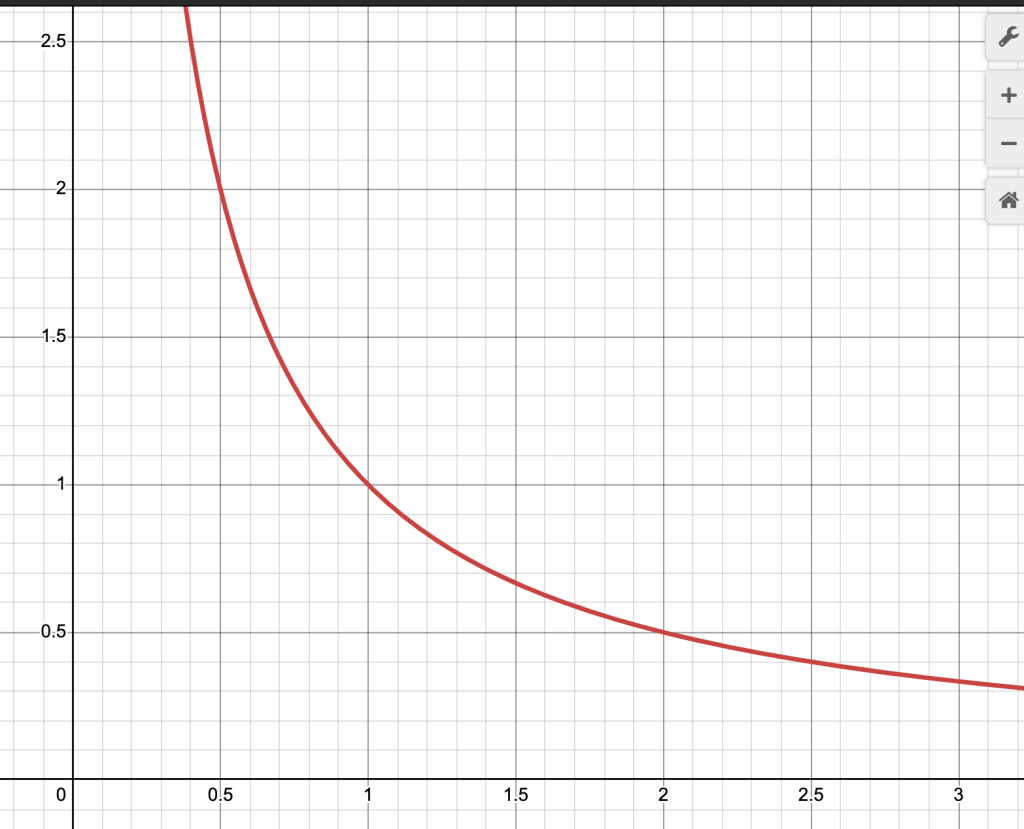
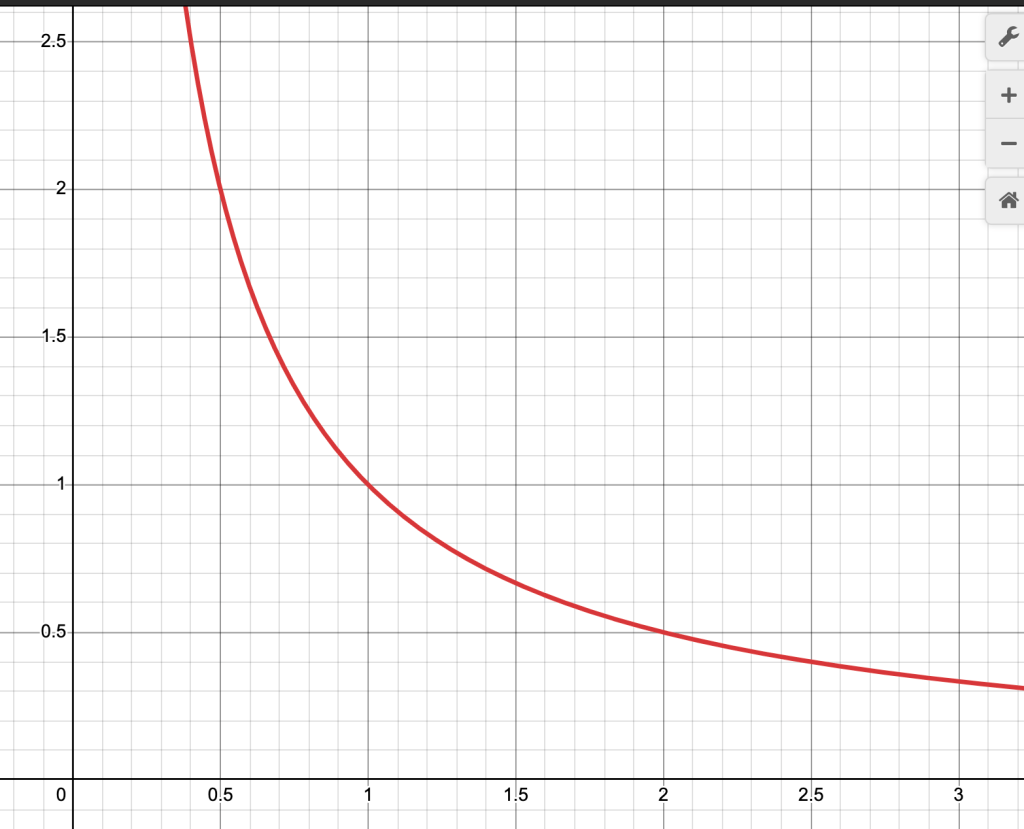
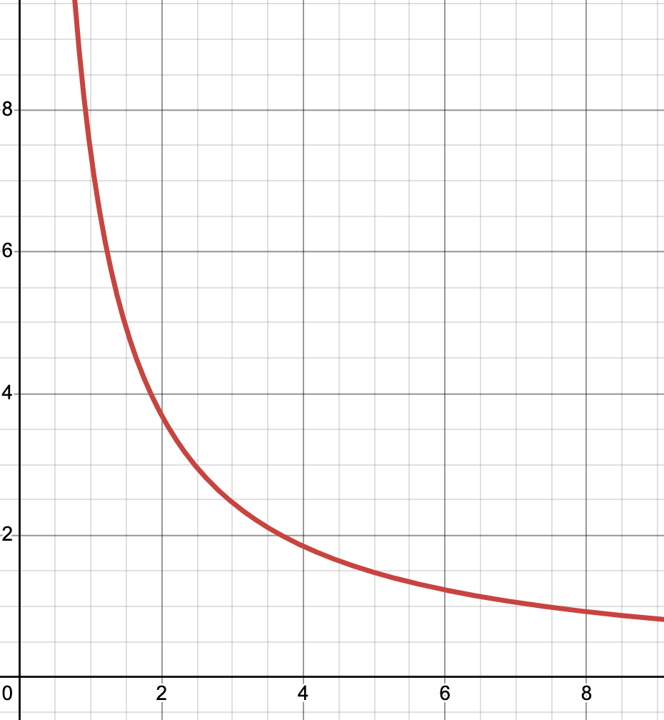
The above graph shows the length on the y-axis and the width on the x axis needed to maintain a constant area of 1 after taking equal but opposite infinitesimal percent changes in each variable. Everywhere in the graph, LxW=1, and L and W are reciprocals.
If we wanted to maintain a constant area for the rectangle of an arbitrary number,
which is 7.389, we have the following:
Note that everywhere in the graph, length on the y-axis and width on the x-axis multiply to 7.389
As shown from the graphs, to maintain a constant area we get hyperbolas.
Since
for various k values we always obtain that W equals the reciprocal of L multiplied by some factor.
This discussion was originally also inspired by a seemingly disparate field: microeconomics. In microeconomics, we study the concept known as elasticity, which measures how sensitive changes in the quantity demanded of a good are to changes in the price of the good.
To measure elasticity, we use the formula:
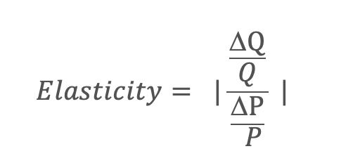
which says given a percentage change in price, how does the quantity demanded change percentage-wise (after taking the absolute value)?
In discussing this concept with some students, we realized that it was impossible to maintain a constant elasticity of 1 when using examples that most books said should give us a constant elasticity of 1 (for example, a 5 % decrease in price that gave rise to a 5% increase in quantity demanded did NOT result in an elasticity of 1 after taking the absolute value, despite the claims of most introductory microeconomics books that it did).
Instead, based on our previous discussion, we now know why this was so: we neglected to adjust for our original price and quantity values, which in reality are constantly changing with each infinitesimal percentage change.
To figure out the equation that allows a constant elasticity of 1, we simply replace L with Q (for quantity) and W with P (for price):
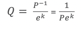
Multiplying each side by P we obtain:
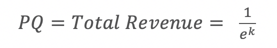
Solving for k when Total Revenue is a constant 1 yields k=0 and would be the same graph showing length and width dimensions when area is 1: